

Ƥ ¼
I ⊥ À I k
I ⊥ þ I k
ð4:122Þ
where I ⊥ and I k are the intensities of the scattered electromagnetic fields perpendicular and parallel to the scattering plane. The degree of linear polarization is usually
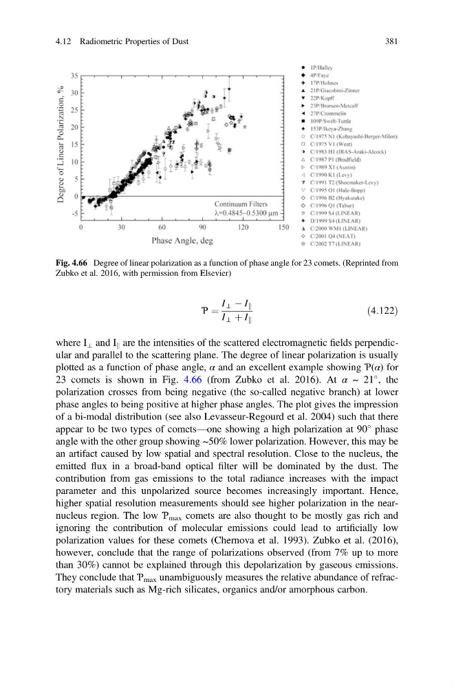
plotted as a function of phase angle, α and an excellent example showing Ƥ(α) for
23 comets is shown in Fig. 4.66 (from Zubko et al. 2016). At α ~ 21
, the
polarization crosses from being negative (the so-called negative branch) at lower
phase angles to being positive at higher phase angles. The plot gives the impression
of a bi-modal distribution (see also Levasseur-Regourd et al. 2004) such that there
appear to be two types of comets—one showing a high polarization at 90
phase
angle with the other group showing ~50% lower polarization. However, this may be
an artifact caused by low spatial and spectral resolution. Close to the nucleus, the
emitted flux in a broad-band optical filter will be dominated by the dust. The
contribution from gas emissions to the total radiance increases with the impact
parameter and this unpolarized source becomes increasingly important. Hence,
higher spatial resolution measurements should see higher polarization in the nearnucleus region. The low Ƥ max comets are also thought to be mostly gas rich and
ignoring the contribution of molecular emissions could lead to artificially low
polarization values for these comets (Chernova et al. 1993). Zubko et al. (2016),
however, conclude that the range of polarizations observed (from 7% up to more
than 30%) cannot be explained through this depolarization by gaseous emissions.
They conclude that Ƥ max unambiguously measures the relative abundance of refractory materials such as Mg-rich silicates, organics and/or amorphous carbon.
Fig. 4.66 Degree of linear polarization as a function of phase angle for 23 comets. (Reprinted from
Zubko et al. 2016, with permission from Elsevier)
4.12 Radiometric Properties of Dust
381
I ⊥ À I k
I ⊥ þ I k
ð4:122Þ
where I ⊥ and I k are the intensities of the scattered electromagnetic fields perpendicular and parallel to the scattering plane. The degree of linear polarization is usually
plotted as a function of phase angle, α and an excellent example showing Ƥ(α) for
23 comets is shown in Fig. 4.66 (from Zubko et al. 2016). At α ~ 21
, the
polarization crosses from being negative (the so-called negative branch) at lower
phase angles to being positive at higher phase angles. The plot gives the impression
of a bi-modal distribution (see also Levasseur-Regourd et al. 2004) such that there
appear to be two types of comets—one showing a high polarization at 90
phase
angle with the other group showing ~50% lower polarization. However, this may be
an artifact caused by low spatial and spectral resolution. Close to the nucleus, the
emitted flux in a broad-band optical filter will be dominated by the dust. The
contribution from gas emissions to the total radiance increases with the impact
parameter and this unpolarized source becomes increasingly important. Hence,
higher spatial resolution measurements should see higher polarization in the nearnucleus region. The low Ƥ max comets are also thought to be mostly gas rich and
ignoring the contribution of molecular emissions could lead to artificially low
polarization values for these comets (Chernova et al. 1993). Zubko et al. (2016),
however, conclude that the range of polarizations observed (from 7% up to more
than 30%) cannot be explained through this depolarization by gaseous emissions.
They conclude that Ƥ max unambiguously measures the relative abundance of refractory materials such as Mg-rich silicates, organics and/or amorphous carbon.
Fig. 4.66 Degree of linear polarization as a function of phase angle for 23 comets. (Reprinted from
Zubko et al. 2016, with permission from Elsevier)
4.12 Radiometric Properties of Dust
381