

f col ¼ σ in v rel n i n n
ð3:116Þ
where v rel is the relative velocity, σ in is the specific ion-neutral cross-section which is
of the order of 10
À19 m
2 and n i and n n define the ion and neutral densities
respectively. The energy transfer to the neutral is then calculated as
E n ¼ 3 k
m i m n
m i þ m n
ð
Þ
2
T i À T n
ð
Þ
ð 3:117Þ
which is a special case of the more general equation for ion-neutral reactions. A
similar equation can be used for electron-neutral elastic collisions by substituting the
terms relating to ions with the analogous terms for electrons. Specific cross-sections
for electron-H 2 O collisions can be found in Itikawa and Mason (2005).
We have seen that fast neutrals can be produced by photodissociation and we
shall see later that ions are accelerated by interaction with the interplanetary magnetic field. These fast species can collide elastically with the bulk fluid to provide
additional heat for the coma and thus modify the reaction chemistry. It is this
phenomenon that drove Rodgers and Charnley, for example, to model the fast
species as independent fluids.
There are also inelastic collisions that need to be accounted for. Collisions may
result in a neutral or ion being lifted into an excited state. That energy can be released
by photon emission which is an energy loss for the species. For the water molecule,
inelastic neutral-neutral collisions remove energy from those neutrals whereas
inelastic electron-neutral collisions result in the removal of energy from the electrons. For H 2 O-H 2 O collisions, Schmidt et al. (1988) have computed the energy
losses (incorporating optical depth effects) whereas the electron energy loss from
electron-H 2 O collisions has been computed by Cravens and Körösmezey (1986).
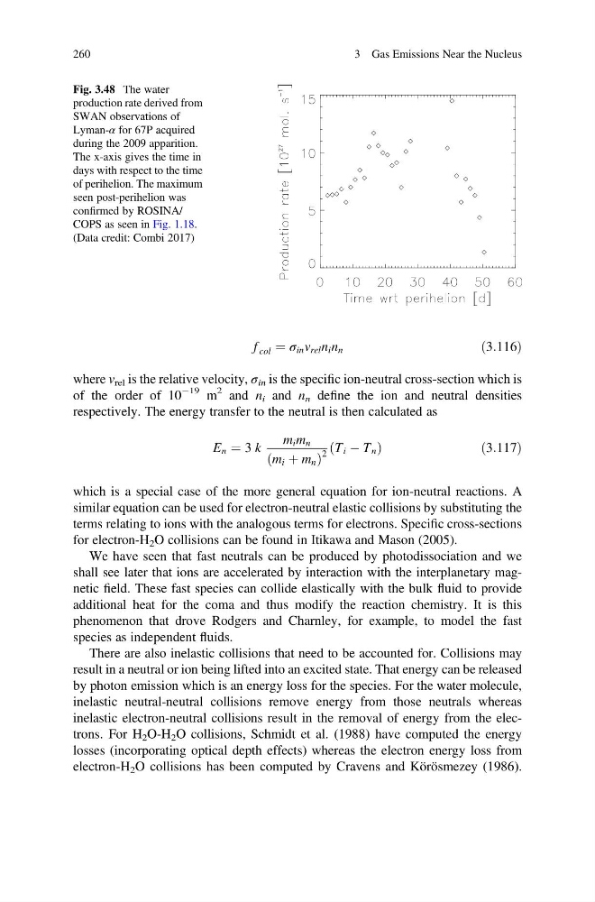
Fig. 3.48 The water
production rate derived from
SWAN observations of
Lyman-α for 67P acquired
during the 2009 apparition.
The x-axis gives the time in
days with respect to the time
of perihelion. The maximum
seen post-perihelion was
confirmed by ROSINA/
COPS as seen in Fig. 1.18.
(Data credit: Combi 2017)
260
3 Gas Emissions Near the Nucleus
ð3:116Þ
where v rel is the relative velocity, σ in is the specific ion-neutral cross-section which is
of the order of 10
À19 m
2 and n i and n n define the ion and neutral densities
respectively. The energy transfer to the neutral is then calculated as
E n ¼ 3 k
m i m n
m i þ m n
ð
Þ
2
T i À T n
ð
Þ
ð 3:117Þ
which is a special case of the more general equation for ion-neutral reactions. A
similar equation can be used for electron-neutral elastic collisions by substituting the
terms relating to ions with the analogous terms for electrons. Specific cross-sections
for electron-H 2 O collisions can be found in Itikawa and Mason (2005).
We have seen that fast neutrals can be produced by photodissociation and we
shall see later that ions are accelerated by interaction with the interplanetary magnetic field. These fast species can collide elastically with the bulk fluid to provide
additional heat for the coma and thus modify the reaction chemistry. It is this
phenomenon that drove Rodgers and Charnley, for example, to model the fast
species as independent fluids.
There are also inelastic collisions that need to be accounted for. Collisions may
result in a neutral or ion being lifted into an excited state. That energy can be released
by photon emission which is an energy loss for the species. For the water molecule,
inelastic neutral-neutral collisions remove energy from those neutrals whereas
inelastic electron-neutral collisions result in the removal of energy from the electrons. For H 2 O-H 2 O collisions, Schmidt et al. (1988) have computed the energy
losses (incorporating optical depth effects) whereas the electron energy loss from
electron-H 2 O collisions has been computed by Cravens and Körösmezey (1986).
Fig. 3.48 The water
production rate derived from
SWAN observations of
Lyman-α for 67P acquired
during the 2009 apparition.
The x-axis gives the time in
days with respect to the time
of perihelion. The maximum
seen post-perihelion was
confirmed by ROSINA/
COPS as seen in Fig. 1.18.
(Data credit: Combi 2017)
260
3 Gas Emissions Near the Nucleus