

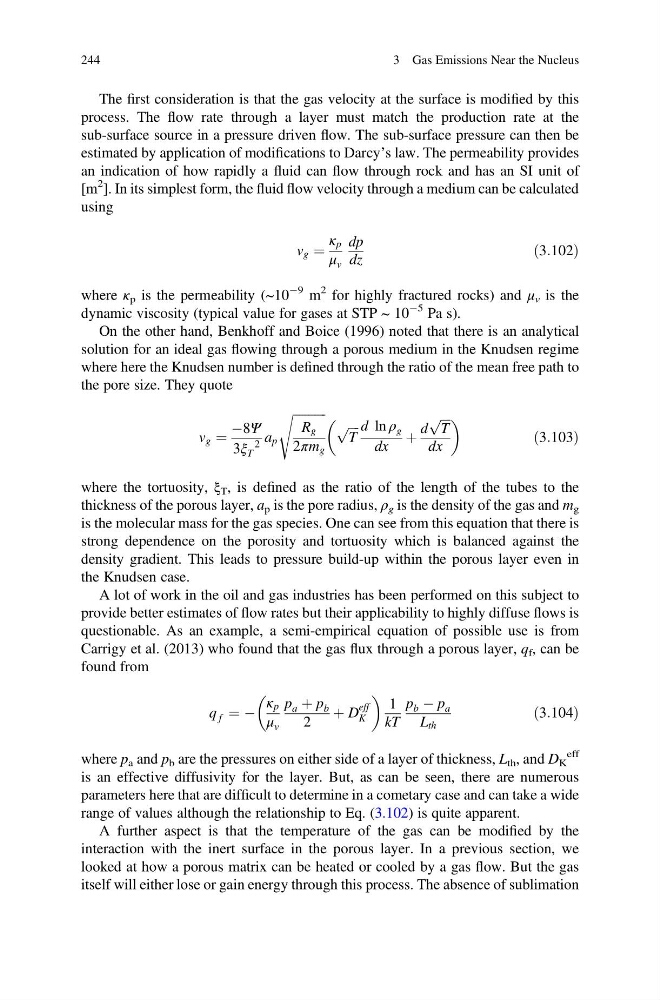
The first consideration is that the gas velocity at the surface is modified by this
process. The flow rate through a layer must match the production rate at the
sub-surface source in a pressure driven flow. The sub-surface pressure can then be
estimated by application of modifications to Darcy’s law. The permeability provides
an indication of how rapidly a fluid can flow through rock and has an SI unit of
[m
2 ]. In its simplest form, the fluid flow velocity through a medium can be calculated
using
v g ¼
κ p
μ v
dp
dz
ð3:102Þ
where κ p is the permeability (~10
À9 m
2 for highly fractured rocks) and μ v is the
dynamic viscosity (typical value for gases at STP ~ 10
À5 Pa s).
On the other hand, Benkhoff and Boice (1996) noted that there is an analytical
solution for an ideal gas flowing through a porous medium in the Knudsen regime
where here the Knudsen number is defined through the ratio of the mean free path to
the pore size. They quote
v g ¼
À8Ψ
3ξ T
2
a p
ffiffiffiffiffiffiffiffiffiffi ffi
R g
2πm g
s
ffiffiffi ffi
T
p d ln ρ g
dx
þ
d
ffiffiffi ffi
T
p
dx
ð3:103Þ
where the tortuosity, ξ T , is defined as the ratio of the length of the tubes to the
thickness of the porous layer, a p is the pore radius, ρ g is the density of the gas and m g
is the molecular mass for the gas species. One can see from this equation that there is
strong dependence on the porosity and tortuosity which is balanced against the
density gradient. This leads to pressure build-up within the porous layer even in
the Knudsen case.
A lot of work in the oil and gas industries has been performed on this subject to
provide better estimates of flow rates but their applicability to highly diffuse flows is
questionable. As an example, a semi-empirical equation of possible use is from
Carrigy et al. (2013) who found that the gas flux through a porous layer, q f , can be
found from
q f ¼ À
κ p
μ v
p a þ p b
2
þ D
eff
K
1
kT
p b À p a
L th
ð3:104Þ
where p a and p b are the pressures on either side of a layer of thickness, L th , and D K
eff
is an effective diffusivity for the layer. But, as can be seen, there are numerous
parameters here that are difficult to determine in a cometary case and can take a wide
range of values although the relationship to Eq. (3.102) is quite apparent.
A further aspect is that the temperature of the gas can be modified by the
interaction with the inert surface in the porous layer. In a previous section, we
looked at how a porous matrix can be heated or cooled by a gas flow. But the gas
itself will either lose or gain energy through this process. The absence of sublimation
244
3 Gas Emissions Near the Nucleus
process. The flow rate through a layer must match the production rate at the
sub-surface source in a pressure driven flow. The sub-surface pressure can then be
estimated by application of modifications to Darcy’s law. The permeability provides
an indication of how rapidly a fluid can flow through rock and has an SI unit of
[m
2 ]. In its simplest form, the fluid flow velocity through a medium can be calculated
using
v g ¼
κ p
μ v
dp
dz
ð3:102Þ
where κ p is the permeability (~10
À9 m
2 for highly fractured rocks) and μ v is the
dynamic viscosity (typical value for gases at STP ~ 10
À5 Pa s).
On the other hand, Benkhoff and Boice (1996) noted that there is an analytical
solution for an ideal gas flowing through a porous medium in the Knudsen regime
where here the Knudsen number is defined through the ratio of the mean free path to
the pore size. They quote
v g ¼
À8Ψ
3ξ T
2
a p
ffiffiffiffiffiffiffiffiffiffi ffi
R g
2πm g
s
ffiffiffi ffi
T
p d ln ρ g
dx
þ
d
ffiffiffi ffi
T
p
dx
ð3:103Þ
where the tortuosity, ξ T , is defined as the ratio of the length of the tubes to the
thickness of the porous layer, a p is the pore radius, ρ g is the density of the gas and m g
is the molecular mass for the gas species. One can see from this equation that there is
strong dependence on the porosity and tortuosity which is balanced against the
density gradient. This leads to pressure build-up within the porous layer even in
the Knudsen case.
A lot of work in the oil and gas industries has been performed on this subject to
provide better estimates of flow rates but their applicability to highly diffuse flows is
questionable. As an example, a semi-empirical equation of possible use is from
Carrigy et al. (2013) who found that the gas flux through a porous layer, q f , can be
found from
q f ¼ À
κ p
μ v
p a þ p b
2
þ D
eff
K
1
kT
p b À p a
L th
ð3:104Þ
where p a and p b are the pressures on either side of a layer of thickness, L th , and D K
eff
is an effective diffusivity for the layer. But, as can be seen, there are numerous
parameters here that are difficult to determine in a cometary case and can take a wide
range of values although the relationship to Eq. (3.102) is quite apparent.
A further aspect is that the temperature of the gas can be modified by the
interaction with the inert surface in the porous layer. In a previous section, we
looked at how a porous matrix can be heated or cooled by a gas flow. But the gas
itself will either lose or gain energy through this process. The absence of sublimation
244
3 Gas Emissions Near the Nucleus