

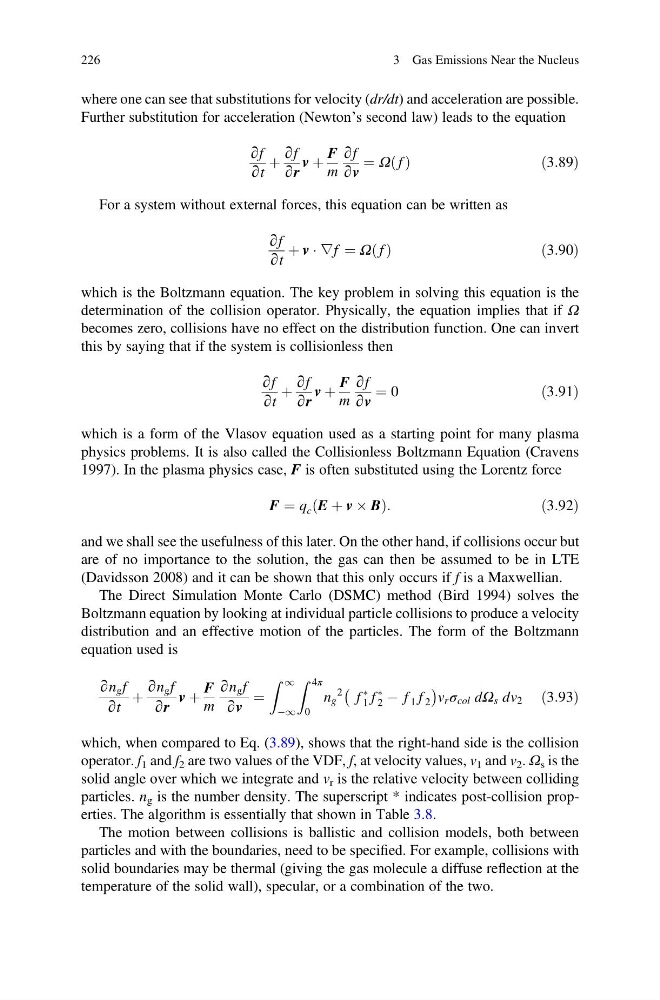
where one can see that substitutions for velocity (dr/dt) and acceleration are possible.
Further substitution for acceleration (Newton’s second law) leads to the equation
∂f
∂t
þ
∂f
∂r
v þ
F
m
∂f
∂v
¼ Ω f
ð Þ
ð3:89Þ
For a system without external forces, this equation can be written as
∂f
∂t
þ v Á ∇f ¼ Ω f
ð Þ
ð3:90Þ
which is the Boltzmann equation. The key problem in solving this equation is the
determination of the collision operator. Physically, the equation implies that if Ω
becomes zero, collisions have no effect on the distribution function. One can invert
this by saying that if the system is collisionless then
∂f
∂t
þ
∂f
∂r
v þ
F
m
∂f
∂v
¼ 0
ð3:91Þ
which is a form of the Vlasov equation used as a starting point for many plasma
physics problems. It is also called the Collisionless Boltzmann Equation (Cravens
1997). In the plasma physics case, F is often substituted using the Lorentz force
F ¼ q c E þ v  B
ð
Þ :
ð3:92Þ
and we shall see the usefulness of this later. On the other hand, if collisions occur but
are of no importance to the solution, the gas can then be assumed to be in LTE
(Davidsson 2008) and it can be shown that this only occurs if f is a Maxwellian.
The Direct Simulation Monte Carlo (DSMC) method (Bird 1994) solves the
Boltzmann equation by looking at individual particle collisions to produce a velocity
distribution and an effective motion of the particles. The form of the Boltzmann
equation used is
∂n g f
∂t
þ
∂n g f
∂r
v þ
F
m
∂n g f
∂v
¼
Z 1
À1
Z 4π
0
n g
2 f
Ã
1 f
Ã
2 À f 1 f 2
À
Á
v r σ col dΩ s dv 2 ð3:93Þ
which, when compared to Eq. (3.89), shows that the right-hand side is the collision
operator. f 1 and f 2 are two values of the VDF, f, at velocity values, v 1 and v 2 . Ω s is the
solid angle over which we integrate and v r is the relative velocity between colliding
particles. n g is the number density. The superscript * indicates post-collision properties. The algorithm is essentially that shown in Table 3.8.
The motion between collisions is ballistic and collision models, both between
particles and with the boundaries, need to be specified. For example, collisions with
solid boundaries may be thermal (giving the gas molecule a diffuse reflection at the
temperature of the solid wall), specular, or a combination of the two.
226
3 Gas Emissions Near the Nucleus
Further substitution for acceleration (Newton’s second law) leads to the equation
∂f
∂t
þ
∂f
∂r
v þ
F
m
∂f
∂v
¼ Ω f
ð Þ
ð3:89Þ
For a system without external forces, this equation can be written as
∂f
∂t
þ v Á ∇f ¼ Ω f
ð Þ
ð3:90Þ
which is the Boltzmann equation. The key problem in solving this equation is the
determination of the collision operator. Physically, the equation implies that if Ω
becomes zero, collisions have no effect on the distribution function. One can invert
this by saying that if the system is collisionless then
∂f
∂t
þ
∂f
∂r
v þ
F
m
∂f
∂v
¼ 0
ð3:91Þ
which is a form of the Vlasov equation used as a starting point for many plasma
physics problems. It is also called the Collisionless Boltzmann Equation (Cravens
1997). In the plasma physics case, F is often substituted using the Lorentz force
F ¼ q c E þ v  B
ð
Þ :
ð3:92Þ
and we shall see the usefulness of this later. On the other hand, if collisions occur but
are of no importance to the solution, the gas can then be assumed to be in LTE
(Davidsson 2008) and it can be shown that this only occurs if f is a Maxwellian.
The Direct Simulation Monte Carlo (DSMC) method (Bird 1994) solves the
Boltzmann equation by looking at individual particle collisions to produce a velocity
distribution and an effective motion of the particles. The form of the Boltzmann
equation used is
∂n g f
∂t
þ
∂n g f
∂r
v þ
F
m
∂n g f
∂v
¼
Z 1
À1
Z 4π
0
n g
2 f
Ã
1 f
Ã
2 À f 1 f 2
À
Á
v r σ col dΩ s dv 2 ð3:93Þ
which, when compared to Eq. (3.89), shows that the right-hand side is the collision
operator. f 1 and f 2 are two values of the VDF, f, at velocity values, v 1 and v 2 . Ω s is the
solid angle over which we integrate and v r is the relative velocity between colliding
particles. n g is the number density. The superscript * indicates post-collision properties. The algorithm is essentially that shown in Table 3.8.
The motion between collisions is ballistic and collision models, both between
particles and with the boundaries, need to be specified. For example, collisions with
solid boundaries may be thermal (giving the gas molecule a diffuse reflection at the
temperature of the solid wall), specular, or a combination of the two.
226
3 Gas Emissions Near the Nucleus