

from the surface, collisions act to change this initial distribution and it evolves into a
Maxwellian equilibrium distribution (Cercignani 2000).
In reality, the VDF at the surface of the nucleus is not known. It is possible to
imagine that the VDF is more collimated or jet-like than a half-Maxwellian if, for
example, gas is ejected through a porous medium at the surface. Distributions such
as cos
x for the VDF (where x can take a value between 1 and 9) have been proposed
for Earth applications. It seems, however, that different assumptions for the VDF
will not produce large differences on the final flow field at comets (Liao et al. 2016)
but it should nonetheless be borne in mind particularly when sources are highly
inhomogeneous.
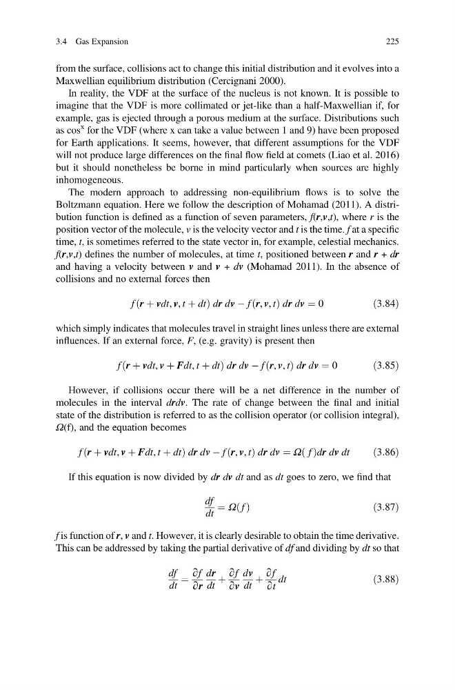
The modern approach to addressing non-equilibrium flows is to solve the
Boltzmann equation. Here we follow the description of Mohamad (2011). A distribution function is defined as a function of seven parameters, f(r,v,t), where r is the
position vector of the molecule, v is the velocity vector and t is the time. f at a specific
time, t, is sometimes referred to the state vector in, for example, celestial mechanics.
f(r,v,t) defines the number of molecules, at time t, positioned between r and r + dr
and having a velocity between v and v + dv (Mohamad 2011). In the absence of
collisions and no external forces then
f r þ vdt, v, t þ dt
ð
Þ dr dv À f r, v, t
ð
Þdr dv ¼ 0
ð3:84Þ
which simply indicates that molecules travel in straight lines unless there are external
influences. If an external force, F, (e.g. gravity) is present then
f r þ vdt, v þ Fdt, t þ dt
ð
Þ dr dv À f r, v, t
ð
Þdr dv ¼ 0
ð3:85Þ
However, if collisions occur there will be a net difference in the number of
molecules in the interval drdv. The rate of change between the final and initial
state of the distribution is referred to as the collision operator (or collision integral),
Ω(f), and the equation becomes
f r þ vdt, v þ Fdt, t þ dt
ð
Þ dr dv À f r, v, t
ð
Þdr dv ¼ Ω f
ð Þdr dv dt
ð3:86Þ
If this equation is now divided by dr dv dt and as dt goes to zero, we find that
df
dt
¼ Ω f
ð Þ
ð3:87Þ
f is function of r, v and t. However, it is clearly desirable to obtain the time derivative.
This can be addressed by taking the partial derivative of df and dividing by dt so that
df
dt
¼
∂f
∂r
dr
dt
þ
∂f
∂v
dv
dt
þ
∂f
∂t
dt
ð3:88Þ
3.4 Gas Expansion
225
Maxwellian equilibrium distribution (Cercignani 2000).
In reality, the VDF at the surface of the nucleus is not known. It is possible to
imagine that the VDF is more collimated or jet-like than a half-Maxwellian if, for
example, gas is ejected through a porous medium at the surface. Distributions such
as cos
x for the VDF (where x can take a value between 1 and 9) have been proposed
for Earth applications. It seems, however, that different assumptions for the VDF
will not produce large differences on the final flow field at comets (Liao et al. 2016)
but it should nonetheless be borne in mind particularly when sources are highly
inhomogeneous.
The modern approach to addressing non-equilibrium flows is to solve the
Boltzmann equation. Here we follow the description of Mohamad (2011). A distribution function is defined as a function of seven parameters, f(r,v,t), where r is the
position vector of the molecule, v is the velocity vector and t is the time. f at a specific
time, t, is sometimes referred to the state vector in, for example, celestial mechanics.
f(r,v,t) defines the number of molecules, at time t, positioned between r and r + dr
and having a velocity between v and v + dv (Mohamad 2011). In the absence of
collisions and no external forces then
f r þ vdt, v, t þ dt
ð
Þ dr dv À f r, v, t
ð
Þdr dv ¼ 0
ð3:84Þ
which simply indicates that molecules travel in straight lines unless there are external
influences. If an external force, F, (e.g. gravity) is present then
f r þ vdt, v þ Fdt, t þ dt
ð
Þ dr dv À f r, v, t
ð
Þdr dv ¼ 0
ð3:85Þ
However, if collisions occur there will be a net difference in the number of
molecules in the interval drdv. The rate of change between the final and initial
state of the distribution is referred to as the collision operator (or collision integral),
Ω(f), and the equation becomes
f r þ vdt, v þ Fdt, t þ dt
ð
Þ dr dv À f r, v, t
ð
Þdr dv ¼ Ω f
ð Þdr dv dt
ð3:86Þ
If this equation is now divided by dr dv dt and as dt goes to zero, we find that
df
dt
¼ Ω f
ð Þ
ð3:87Þ
f is function of r, v and t. However, it is clearly desirable to obtain the time derivative.
This can be addressed by taking the partial derivative of df and dividing by dt so that
df
dt
¼
∂f
∂r
dr
dt
þ
∂f
∂v
dv
dt
þ
∂f
∂t
dt
ð3:88Þ
3.4 Gas Expansion
225