

conductivity can be described (see Russell 1935; Espinasse et al. 1993; Marboeuf
et al. 2012) as
κ m ¼
κ s Ψ
2=3
κ p þ κ s 1 À Ψ
2=3
À
Á
Â
Ã
κ s Ψ À Ψ
2=3
þ 1
Â
à À κ p Ψ
2=3
Ψ
1=3
À 1
Â
Ã
ð2:117Þ
where κ p is the radiative conductivity across the pores as described by Squyres et al.
(1985) through the equation
κ p ¼ 4εσr p T
3
ð2:118Þ
and κ s is the conductivity of the solid phase of the components which can be the
result of a mixture of materials with individual conductivities (Marboeuf et al. 2012).
Laboratory measurements of the thermal conductivity of porous but consolidated
materials are now fairly commonplace using hot plates or methods such as the
transient hot wire technique (e.g. Smith et al. 2013). However, measurements of
fragile, porous, dust aggregates in the laboratory is not trivial. Techniques have been
developed by Krause et al. (2011) using the thermal IR emission observed following
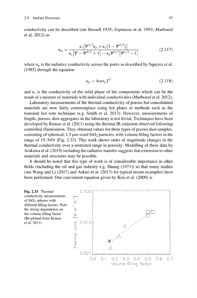
controlled illumination. They obtained values for three types of porous dust samples,
consisting of spherical, 1.5 μm-sized SiO 2 particles, with volume filling factors in the
range of 15–54% (Fig. 2.33). This work shows order of magnitude changes in the
thermal conductivity over a restricted range in porosity. Modelling of these data by
Arakawa et al. (2019) including the radiative transfer suggests that extension to other
materials and structures may be possible.
It should be noted that this type of work is of considerable importance in other
fields (including the oil and gas industry e.g. Huang (1971)) so that many studies
(see Wang and Li (2017) and Askari et al. (2017) for typical recent examples) have
been performed. One convenient equation given by Kou et al. (2009) is
Fig. 2.33 Thermal
conductivity measurements
of SiO 2 spheres with
different filling factors. Note
the strong dependence on
the volume filling factor
(Re-plotted from Krause
et al. 2011)
2.9 Surface Processes
97
et al. 2012) as
κ m ¼
κ s Ψ
2=3
κ p þ κ s 1 À Ψ
2=3
À
Á
Â
Ã
κ s Ψ À Ψ
2=3
þ 1
Â
à À κ p Ψ
2=3
Ψ
1=3
À 1
Â
Ã
ð2:117Þ
where κ p is the radiative conductivity across the pores as described by Squyres et al.
(1985) through the equation
κ p ¼ 4εσr p T
3
ð2:118Þ
and κ s is the conductivity of the solid phase of the components which can be the
result of a mixture of materials with individual conductivities (Marboeuf et al. 2012).
Laboratory measurements of the thermal conductivity of porous but consolidated
materials are now fairly commonplace using hot plates or methods such as the
transient hot wire technique (e.g. Smith et al. 2013). However, measurements of
fragile, porous, dust aggregates in the laboratory is not trivial. Techniques have been
developed by Krause et al. (2011) using the thermal IR emission observed following
controlled illumination. They obtained values for three types of porous dust samples,
consisting of spherical, 1.5 μm-sized SiO 2 particles, with volume filling factors in the
range of 15–54% (Fig. 2.33). This work shows order of magnitude changes in the
thermal conductivity over a restricted range in porosity. Modelling of these data by
Arakawa et al. (2019) including the radiative transfer suggests that extension to other
materials and structures may be possible.
It should be noted that this type of work is of considerable importance in other
fields (including the oil and gas industry e.g. Huang (1971)) so that many studies
(see Wang and Li (2017) and Askari et al. (2017) for typical recent examples) have
been performed. One convenient equation given by Kou et al. (2009) is
Fig. 2.33 Thermal
conductivity measurements
of SiO 2 spheres with
different filling factors. Note
the strong dependence on
the volume filling factor
(Re-plotted from Krause
et al. 2011)
2.9 Surface Processes
97