

4 QCD: The Theory of Strong Interactions
93
and the wave function renormalisation factors Z
1/2
q,g for q and g, using suitable
renormalisation conditions (that is precise definitions of m, g and Z that can be
implemented order by order in perturbation theory). For example we can define
the renormalised mass m as the position of the pole in the quark propagator and,
similarly, the normalisation Z q as the residue at the pole:
Propagator =
Z q
p 2 − m 2 + no − pole terms
(4.15)
The renormalised coupling e can be defined in terms of a renormalised 3-point
vertex at some specified values of the external momenta. Precisely, we consider
a one particle irreducible vertex (1PI). We recall that a connected Green function
is the sum of all connected diagrams, while 1PI Green functions are the sum of all
diagrams that cannot be separated into two disconnected parts by cutting only one
line.
We now become more specific by concentrating on the case of massless QCD. If
we start from a vanishing mass at the classical (or “bare”) level, m 0 = 0, the mass
is not renormalised because it is protected by a symmetry, chiral symmetry. The
conserved currents of chiral symmetry are axial currents: ¯
qγ μ γ 5 q. The divergence
of the axial current gives, by using the Dirac equation, ∂ μ ( ¯
qγ μ γ 5 q) = 2m ¯
qγ 5 q. So
the axial current and the corresponding axial charge are conserved in the massless
limit. Since QCD is a vector theory we have not to worry about chiral anomalies
in this respect. So one can choose a regularisation that preserves chiral symmetry
besides gauge and Lorentz symmetry. Then the renormalised mass remains zero.
The renormalised propagator has the form in Eq. (4.15) with m = 0.
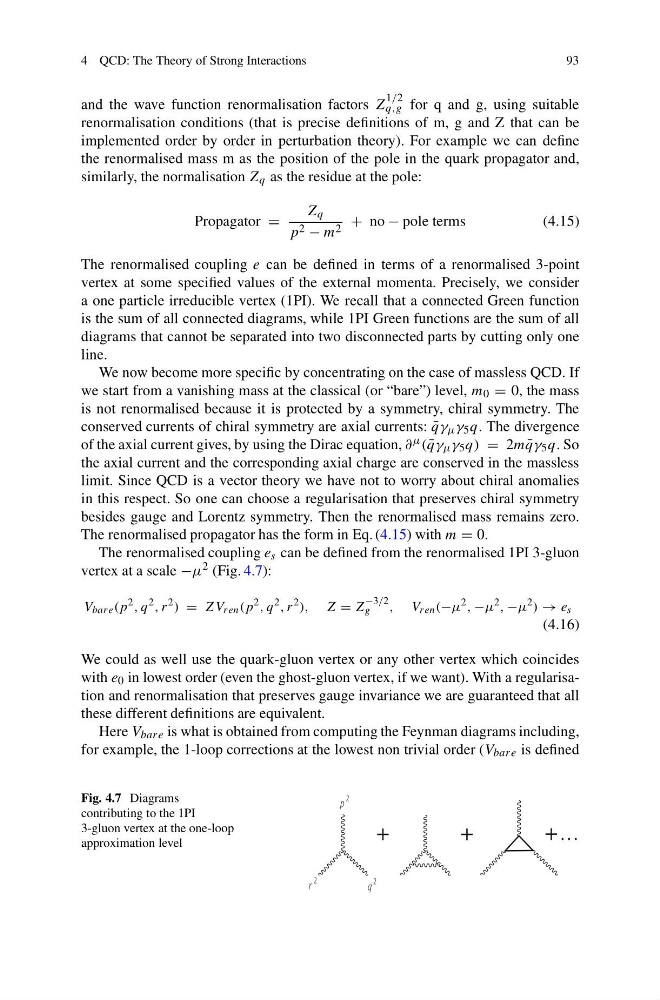
The renormalised coupling e s can be defined from the renormalised 1PI 3-gluon
vertex at a scale −μ 2 (Fig. 4.7):
V bare (p
2 , q
2 , r
2 ) = ZV ren (p
2 , q
2 , r
2 ), Z = Z
−3/2
g
, V ren (−μ
2 , −μ
2 , −μ
2 ) → e s
(4.16)
We could as well use the quark-gluon vertex or any other vertex which coincides
with e 0 in lowest order (even the ghost-gluon vertex, if we want). With a regularisation and renormalisation that preserves gauge invariance we are guaranteed that all
these different definitions are equivalent.
Here V bare is what is obtained from computing the Feynman diagrams including,
for example, the 1-loop corrections at the lowest non trivial order (V bare is defined
Fig. 4.7 Diagrams
contributing to the 1PI
3-gluon vertex at the one-loop
approximation level
+
+
+...
p
2
q
2
r
2
93
and the wave function renormalisation factors Z
1/2
q,g for q and g, using suitable
renormalisation conditions (that is precise definitions of m, g and Z that can be
implemented order by order in perturbation theory). For example we can define
the renormalised mass m as the position of the pole in the quark propagator and,
similarly, the normalisation Z q as the residue at the pole:
Propagator =
Z q
p 2 − m 2 + no − pole terms
(4.15)
The renormalised coupling e can be defined in terms of a renormalised 3-point
vertex at some specified values of the external momenta. Precisely, we consider
a one particle irreducible vertex (1PI). We recall that a connected Green function
is the sum of all connected diagrams, while 1PI Green functions are the sum of all
diagrams that cannot be separated into two disconnected parts by cutting only one
line.
We now become more specific by concentrating on the case of massless QCD. If
we start from a vanishing mass at the classical (or “bare”) level, m 0 = 0, the mass
is not renormalised because it is protected by a symmetry, chiral symmetry. The
conserved currents of chiral symmetry are axial currents: ¯
qγ μ γ 5 q. The divergence
of the axial current gives, by using the Dirac equation, ∂ μ ( ¯
qγ μ γ 5 q) = 2m ¯
qγ 5 q. So
the axial current and the corresponding axial charge are conserved in the massless
limit. Since QCD is a vector theory we have not to worry about chiral anomalies
in this respect. So one can choose a regularisation that preserves chiral symmetry
besides gauge and Lorentz symmetry. Then the renormalised mass remains zero.
The renormalised propagator has the form in Eq. (4.15) with m = 0.
The renormalised coupling e s can be defined from the renormalised 1PI 3-gluon
vertex at a scale −μ 2 (Fig. 4.7):
V bare (p
2 , q
2 , r
2 ) = ZV ren (p
2 , q
2 , r
2 ), Z = Z
−3/2
g
, V ren (−μ
2 , −μ
2 , −μ
2 ) → e s
(4.16)
We could as well use the quark-gluon vertex or any other vertex which coincides
with e 0 in lowest order (even the ghost-gluon vertex, if we want). With a regularisation and renormalisation that preserves gauge invariance we are guaranteed that all
these different definitions are equivalent.
Here V bare is what is obtained from computing the Feynman diagrams including,
for example, the 1-loop corrections at the lowest non trivial order (V bare is defined
Fig. 4.7 Diagrams
contributing to the 1PI
3-gluon vertex at the one-loop
approximation level
+
+
+...
p
2
q
2
r
2