

7 Relativistic Nucleus-Nucleus Collisions and the QCD Matter Phase Diagram
357
be determined separately), and the flow pattern drops out from the yield distribution
over species in 4π acceptance [110]. For nuclear collisions at SPS energies and
below one thus should perform a SHM analysis of the total, 4π-integrated hadronic
multiplicities, as was done in Fig. 7.25.
We note that the derivation above illustrates the termination problem of the
hydrodynamic description of A+A collisions, the validity of which depends on
conditions of a short mean free path, λ < 1 fm. A precise argumentation suggests
that two different free paths are relevant here, concerning hadron occupation number
and hadron spectral freeze-out, respectively. As hadrochemical freeze-out occurs in
the immediate vicinity of T c (and T H ≈ 160–165 MeV from Figs. 7.25 and 7.26), the
hadron species distribution stays constant throughout the ensuing hadronic phase,
i.e. the “chemical” mean free path abruptly becomes infinite at T H , whereas elastic
and resonant rescattering may well extend far into the hadronic phase, and so does
collective pressure and flow. In fact we have seen in Sect. 7.2.6 that the decoupling
from flow occurs at T F as low as 90–100 MeV (Fig. 7.24). Thus the hydrodynamic
evolution of high
√
s collisions has to be, somehow artificially, stopped at the
parton-hadron boundary in order to get the correct hadron multiplicities N i , of
Eqs. (7.26)–(7.29), which then stay frozen-out during the subsequent hadronic
expansion.
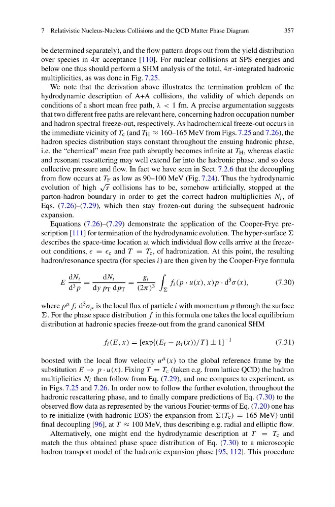
Equations (7.26)–(7.29) demonstrate the application of the Cooper-Frye prescription [111] for termination of the hydrodynamic evolution. The hyper-surface
describes the space-time location at which individual flow cells arrive at the freezeout conditions, = c and T = T c , of hadronization. At this point, the resulting
hadron/resonance spectra (for species i) are then given by the Cooper-Frye formula
E
dN i
d 3 p
=
dN i
dy p T dp T
=
g i
(2π) 3
f i (p · u(x), x)p · d
3 σ (x),
(7.30)
where p μ f i d 3 σ μ is the local flux of particle i with momentum p through the surface
. For the phase space distribution f in this formula one takes the local equilibrium
distribution at hadronic species freeze-out from the grand canonical SHM
f i (E, x) = [exp{(E i − μ i (x))/T } ± 1]
−1
(7.31)
boosted with the local flow velocity u μ (x) to the global reference frame by the
substitution E → p · u(x). Fixing T = T c (taken e.g. from lattice QCD) the hadron
multiplicities N i then follow from Eq. (7.29), and one compares to experiment, as
in Figs. 7.25 and 7.26. In order now to follow the further evolution, throughout the
hadronic rescattering phase, and to finally compare predictions of Eq. (7.30) to the
observed flow data as represented by the various Fourier-terms of Eq. (7.20) one has
to re-initialize (with hadronic EOS) the expansion from (T c ) = 165 MeV) until
final decoupling [96], at T ≈ 100 MeV, thus describing e.g. radial and elliptic flow.
Alternatively, one might end the hydrodynamic description at T = T c and
match the thus obtained phase space distribution of Eq. (7.30) to a microscopic
hadron transport model of the hadronic expansion phase [95, 112]. This procedure
357
be determined separately), and the flow pattern drops out from the yield distribution
over species in 4π acceptance [110]. For nuclear collisions at SPS energies and
below one thus should perform a SHM analysis of the total, 4π-integrated hadronic
multiplicities, as was done in Fig. 7.25.
We note that the derivation above illustrates the termination problem of the
hydrodynamic description of A+A collisions, the validity of which depends on
conditions of a short mean free path, λ < 1 fm. A precise argumentation suggests
that two different free paths are relevant here, concerning hadron occupation number
and hadron spectral freeze-out, respectively. As hadrochemical freeze-out occurs in
the immediate vicinity of T c (and T H ≈ 160–165 MeV from Figs. 7.25 and 7.26), the
hadron species distribution stays constant throughout the ensuing hadronic phase,
i.e. the “chemical” mean free path abruptly becomes infinite at T H , whereas elastic
and resonant rescattering may well extend far into the hadronic phase, and so does
collective pressure and flow. In fact we have seen in Sect. 7.2.6 that the decoupling
from flow occurs at T F as low as 90–100 MeV (Fig. 7.24). Thus the hydrodynamic
evolution of high
√
s collisions has to be, somehow artificially, stopped at the
parton-hadron boundary in order to get the correct hadron multiplicities N i , of
Eqs. (7.26)–(7.29), which then stay frozen-out during the subsequent hadronic
expansion.
Equations (7.26)–(7.29) demonstrate the application of the Cooper-Frye prescription [111] for termination of the hydrodynamic evolution. The hyper-surface
describes the space-time location at which individual flow cells arrive at the freezeout conditions, = c and T = T c , of hadronization. At this point, the resulting
hadron/resonance spectra (for species i) are then given by the Cooper-Frye formula
E
dN i
d 3 p
=
dN i
dy p T dp T
=
g i
(2π) 3
f i (p · u(x), x)p · d
3 σ (x),
(7.30)
where p μ f i d 3 σ μ is the local flux of particle i with momentum p through the surface
. For the phase space distribution f in this formula one takes the local equilibrium
distribution at hadronic species freeze-out from the grand canonical SHM
f i (E, x) = [exp{(E i − μ i (x))/T } ± 1]
−1
(7.31)
boosted with the local flow velocity u μ (x) to the global reference frame by the
substitution E → p · u(x). Fixing T = T c (taken e.g. from lattice QCD) the hadron
multiplicities N i then follow from Eq. (7.29), and one compares to experiment, as
in Figs. 7.25 and 7.26. In order now to follow the further evolution, throughout the
hadronic rescattering phase, and to finally compare predictions of Eq. (7.30) to the
observed flow data as represented by the various Fourier-terms of Eq. (7.20) one has
to re-initialize (with hadronic EOS) the expansion from (T c ) = 165 MeV) until
final decoupling [96], at T ≈ 100 MeV, thus describing e.g. radial and elliptic flow.
Alternatively, one might end the hydrodynamic description at T = T c and
match the thus obtained phase space distribution of Eq. (7.30) to a microscopic
hadron transport model of the hadronic expansion phase [95, 112]. This procedure