

122
G. Altarelli and S. Forte
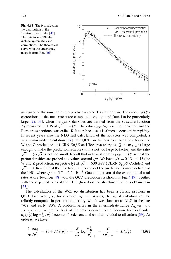
Fig. 4.18 The b production
p T distribution at the
Tevatron p ¯
p collider [47].
The data from CDF also
include systematics and
correlations. The theoretical
curve with the uncertainty
range is from Ref. [46]
antiquark of the same colour to produce a colourless lepton pair. The order α s (Q 2 )
corrections to the total rate were computed long ago and found to be particularly
large [22, 38], when the quark densities are defined from the structure function
F 2 measured in DIS at q 2 = −Q 2 . The ratio σ corr /σ LO of the corrected and the
Born cross-sections, was called K-factor, because it is almost a constant in rapidity.
In recent years also the NLO full calculation of the K-factor was completed, a
very remarkable calculation [37]. The QCD predictions have been best tested for
W and Z production at CERN Sp ¯
pS and Tevatron energies. Q ∼ m W,Z is large
enough to make the prediction reliable (with a not too large K-factor) and the ratio
√
τ = Q/
√
s is not too small. Recall that in lowest order x 1 x 2 s = Q 2 so that the
parton densities are probed at x values around
√
τ . We have
√
τ = 0.13 − 0.15 (for
W and Z production, respectively) at
√
s = 630 GeV (CERN Sp ¯
pS Collider) and
√
τ = 0.04 − 0.05 at the Tevatron. In this respect the prediction is more delicate at
the LHC, where
√
τ ∼ 5.7 − 6.5 · 10 −3 . One comparison of the experimental total
rates at the Tevatron [48] with the QCD predictions is shown in Fig. 4.19, together
with the expected rates at the LHC (based on the structure functions obtained in
[23]).
The calculation of the W/Z p T distribution has been a classic problem in
QCD. For large p T , for example p T ∼ o(m W ), the p T distribution can be
reliably computed in perturbation theory, which was done up to NLO in the late
‘70’s and early ‘80’s. A problem arises in the intermediate range QCD <<
p T << m W , where the bulk of the data is concentrated, because terms of order
α s (p 2
T ) log m 2
W /p 2
T become of order one and should included to all orders [39]. At
order α s we have:
1
σ 0
dσ 0
dp 2
T
= (1 + A)δ(p
2
T ) +
B
p 2
T
log
m 2
W
p 2
T +
+
C
(p 2
T ) +
+ D(p
2
T )
(4.98)
G. Altarelli and S. Forte
Fig. 4.18 The b production
p T distribution at the
Tevatron p ¯
p collider [47].
The data from CDF also
include systematics and
correlations. The theoretical
curve with the uncertainty
range is from Ref. [46]
antiquark of the same colour to produce a colourless lepton pair. The order α s (Q 2 )
corrections to the total rate were computed long ago and found to be particularly
large [22, 38], when the quark densities are defined from the structure function
F 2 measured in DIS at q 2 = −Q 2 . The ratio σ corr /σ LO of the corrected and the
Born cross-sections, was called K-factor, because it is almost a constant in rapidity.
In recent years also the NLO full calculation of the K-factor was completed, a
very remarkable calculation [37]. The QCD predictions have been best tested for
W and Z production at CERN Sp ¯
pS and Tevatron energies. Q ∼ m W,Z is large
enough to make the prediction reliable (with a not too large K-factor) and the ratio
√
τ = Q/
√
s is not too small. Recall that in lowest order x 1 x 2 s = Q 2 so that the
parton densities are probed at x values around
√
τ . We have
√
τ = 0.13 − 0.15 (for
W and Z production, respectively) at
√
s = 630 GeV (CERN Sp ¯
pS Collider) and
√
τ = 0.04 − 0.05 at the Tevatron. In this respect the prediction is more delicate at
the LHC, where
√
τ ∼ 5.7 − 6.5 · 10 −3 . One comparison of the experimental total
rates at the Tevatron [48] with the QCD predictions is shown in Fig. 4.19, together
with the expected rates at the LHC (based on the structure functions obtained in
[23]).
The calculation of the W/Z p T distribution has been a classic problem in
QCD. For large p T , for example p T ∼ o(m W ), the p T distribution can be
reliably computed in perturbation theory, which was done up to NLO in the late
‘70’s and early ‘80’s. A problem arises in the intermediate range QCD <<
p T << m W , where the bulk of the data is concentrated, because terms of order
α s (p 2
T ) log m 2
W /p 2
T become of order one and should included to all orders [39]. At
order α s we have:
1
σ 0
dσ 0
dp 2
T
= (1 + A)δ(p
2
T ) +
B
p 2
T
log
m 2
W
p 2
T +
+
C
(p 2
T ) +
+ D(p
2
T )
(4.98)