

114
G. Altarelli and S. Forte
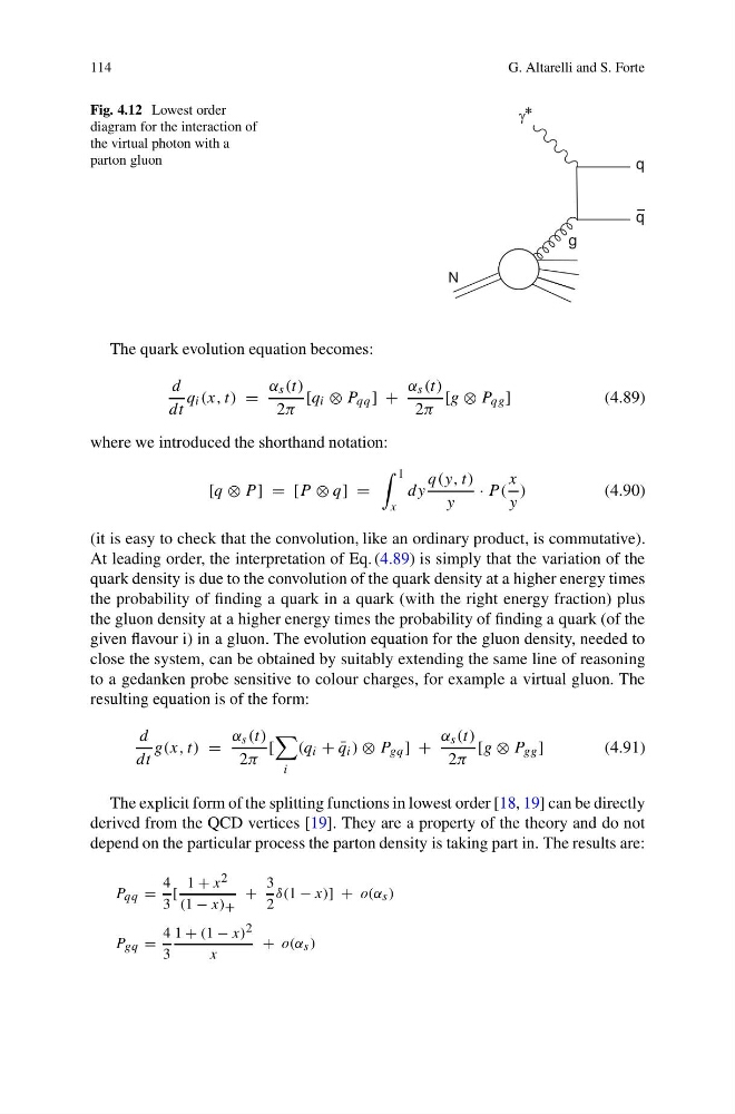
Fig. 4.12 Lowest order
diagram for the interaction of
the virtual photon with a
parton gluon
q
q
g
J
N
*
The quark evolution equation becomes:
d
dt
q i (x, t) =
α s (t)
2π
[q i ⊗ P qq ] +
α s (t)
2π
[g ⊗ P qg ]
(4.89)
where we introduced the shorthand notation:
[q ⊗ P ] = [P ⊗ q] =
1
x
dy
q(y, t)
y
· P (
x
y
)
(4.90)
(it is easy to check that the convolution, like an ordinary product, is commutative).
At leading order, the interpretation of Eq. (4.89) is simply that the variation of the
quark density is due to the convolution of the quark density at a higher energy times
the probability of finding a quark in a quark (with the right energy fraction) plus
the gluon density at a higher energy times the probability of finding a quark (of the
given flavour i) in a gluon. The evolution equation for the gluon density, needed to
close the system, can be obtained by suitably extending the same line of reasoning
to a gedanken probe sensitive to colour charges, for example a virtual gluon. The
resulting equation is of the form:
d
dt
g(x, t) =
α s (t)
2π
[
i
(q i + ¯
q i ) ⊗ P gq ] +
α s (t)
2π
[g ⊗ P gg ]
(4.91)
The explicit form of the splitting functions in lowest order [18, 19] can be directly
derived from the QCD vertices [19]. They are a property of the theory and do not
depend on the particular process the parton density is taking part in. The results are:
P qq =
4
3
[
1 + x 2
(1 − x) +
+
3
2
δ(1 − x)] + o(α s )
P gq =
4
3
1 + (1 − x) 2
x
+ o(α s )
G. Altarelli and S. Forte
Fig. 4.12 Lowest order
diagram for the interaction of
the virtual photon with a
parton gluon
q
q
g
J
N
*
The quark evolution equation becomes:
d
dt
q i (x, t) =
α s (t)
2π
[q i ⊗ P qq ] +
α s (t)
2π
[g ⊗ P qg ]
(4.89)
where we introduced the shorthand notation:
[q ⊗ P ] = [P ⊗ q] =
1
x
dy
q(y, t)
y
· P (
x
y
)
(4.90)
(it is easy to check that the convolution, like an ordinary product, is commutative).
At leading order, the interpretation of Eq. (4.89) is simply that the variation of the
quark density is due to the convolution of the quark density at a higher energy times
the probability of finding a quark in a quark (with the right energy fraction) plus
the gluon density at a higher energy times the probability of finding a quark (of the
given flavour i) in a gluon. The evolution equation for the gluon density, needed to
close the system, can be obtained by suitably extending the same line of reasoning
to a gedanken probe sensitive to colour charges, for example a virtual gluon. The
resulting equation is of the form:
d
dt
g(x, t) =
α s (t)
2π
[
i
(q i + ¯
q i ) ⊗ P gq ] +
α s (t)
2π
[g ⊗ P gg ]
(4.91)
The explicit form of the splitting functions in lowest order [18, 19] can be directly
derived from the QCD vertices [19]. They are a property of the theory and do not
depend on the particular process the parton density is taking part in. The results are:
P qq =
4
3
[
1 + x 2
(1 − x) +
+
3
2
δ(1 − x)] + o(α s )
P gq =
4
3
1 + (1 − x) 2
x
+ o(α s )