

40
H. Bichsel and H. Schindler
0
50
100
m]
μ
[
x
0
0.1
0.2
[a. u.]
x
/d
e
n
d
p
R
0.95
R
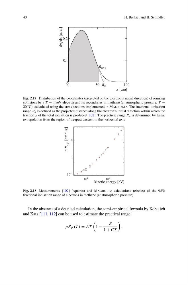
Fig. 2.17 Distribution of the coordinates (projected on the electron’s initial direction) of ionising
collisions by a T = 1 keV electron and its secondaries in methane (at atmospheric pressure, T =
20 ◦ C), calculated using the cross sections implemented in MAGBOLTZ. The fractional ionisation
range R x is defined as the projected distance along the electron’s initial direction within which the
fraction x of the total ionisation is produced [102]. The practical range R p is determined by linear
extrapolation from the region of steepest descent to the horizontal axis
2
10
3
10
kinetic energy [eV]
1
−
10
1
10
g]
μ
-2
[cm
0.95
R
ρ
Fig. 2.18 Measurements [102] (squares) and MAGBOLTZ calculations (circles) of the 95%
fractional ionisation range of electrons in methane (at atmospheric pressure)
In the absence of a detailed calculation, the semi-empirical formula by Kobetich
and Katz [111, 112] can be used to estimate the practical range,
ρR p (T ) = AT
1 −
B
1 + CT
,
H. Bichsel and H. Schindler
0
50
100
m]
μ
[
x
0
0.1
0.2
[a. u.]
x
/d
e
n
d
p
R
0.95
R
Fig. 2.17 Distribution of the coordinates (projected on the electron’s initial direction) of ionising
collisions by a T = 1 keV electron and its secondaries in methane (at atmospheric pressure, T =
20 ◦ C), calculated using the cross sections implemented in MAGBOLTZ. The fractional ionisation
range R x is defined as the projected distance along the electron’s initial direction within which the
fraction x of the total ionisation is produced [102]. The practical range R p is determined by linear
extrapolation from the region of steepest descent to the horizontal axis
2
10
3
10
kinetic energy [eV]
1
−
10
1
10
g]
μ
-2
[cm
0.95
R
ρ
Fig. 2.18 Measurements [102] (squares) and MAGBOLTZ calculations (circles) of the 95%
fractional ionisation range of electrons in methane (at atmospheric pressure)
In the absence of a detailed calculation, the semi-empirical formula by Kobetich
and Katz [111, 112] can be used to estimate the practical range,
ρR p (T ) = AT
1 −
B
1 + CT
,