

36
H. Bichsel and H. Schindler
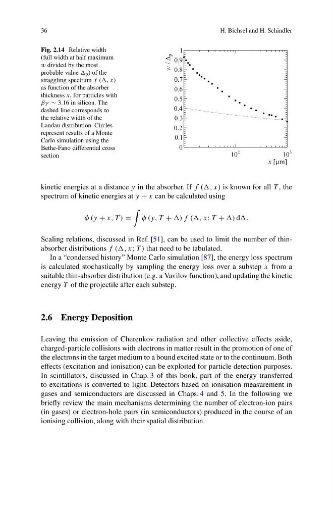
Fig. 2.14 Relative width
(full width at half maximum
w divided by the most
probable value p ) of the
straggling spectrum f ((, x)
as function of the absorber
thickness x, for particles with
βγ ∼ 3.16 in silicon. The
dashed line corresponds to
the relative width of the
Landau distribution. Circles
represent results of a Monte
Carlo simulation using the
Bethe-Fano differential cross
section
2
10
3
10
x [μm]
0
0.1
0.2
0.3
0.4
0.5
0.6
0.7
0.8
0.9
1
w /
Δ
p
kinetic energies at a distance y in the absorber. If f (, x) is known for all T , the
spectrum of kinetic energies at y + x can be calculated using
φ (y + x, T ) =
φ (y, T + ) f ( x; T + ) d.
Scaling relations, discussed in Ref. [51], can be used to limit the number of thinabsorber distributions f ( x; T ) that need to be tabulated.
In a “condensed history” Monte Carlo simulation [87], the energy loss spectrum
is calculated stochastically by sampling the energy loss over a substep x from a
suitable thin-absorber distribution (e.g. a Vavilov function), and updating the kinetic
energy T of the projectile after each substep.
2.6 Energy Deposition
Leaving the emission of Cherenkov radiation and other collective effects aside,
charged-particle collisions with electrons in matter result in the promotion of one of
the electrons in the target medium to a bound excited state or to the continuum. Both
effects (excitation and ionisation) can be exploited for particle detection purposes.
In scintillators, discussed in Chap. 3 of this book, part of the energy transferred
to excitations is converted to light. Detectors based on ionisation measurement in
gases and semiconductors are discussed in Chaps. 4 and 5. In the following we
briefly review the main mechanisms determining the number of electron-ion pairs
(in gases) or electron-hole pairs (in semiconductors) produced in the course of an
ionising collision, along with their spatial distribution.
H. Bichsel and H. Schindler
Fig. 2.14 Relative width
(full width at half maximum
w divided by the most
probable value p ) of the
straggling spectrum f ((, x)
as function of the absorber
thickness x, for particles with
βγ ∼ 3.16 in silicon. The
dashed line corresponds to
the relative width of the
Landau distribution. Circles
represent results of a Monte
Carlo simulation using the
Bethe-Fano differential cross
section
2
10
3
10
x [μm]
0
0.1
0.2
0.3
0.4
0.5
0.6
0.7
0.8
0.9
1
w /
Δ
p
kinetic energies at a distance y in the absorber. If f (, x) is known for all T , the
spectrum of kinetic energies at y + x can be calculated using
φ (y + x, T ) =
φ (y, T + ) f ( x; T + ) d.
Scaling relations, discussed in Ref. [51], can be used to limit the number of thinabsorber distributions f ( x; T ) that need to be tabulated.
In a “condensed history” Monte Carlo simulation [87], the energy loss spectrum
is calculated stochastically by sampling the energy loss over a substep x from a
suitable thin-absorber distribution (e.g. a Vavilov function), and updating the kinetic
energy T of the projectile after each substep.
2.6 Energy Deposition
Leaving the emission of Cherenkov radiation and other collective effects aside,
charged-particle collisions with electrons in matter result in the promotion of one of
the electrons in the target medium to a bound excited state or to the continuum. Both
effects (excitation and ionisation) can be exploited for particle detection purposes.
In scintillators, discussed in Chap. 3 of this book, part of the energy transferred
to excitations is converted to light. Detectors based on ionisation measurement in
gases and semiconductors are discussed in Chaps. 4 and 5. In the following we
briefly review the main mechanisms determining the number of electron-ion pairs
(in gases) or electron-hole pairs (in semiconductors) produced in the course of an
ionising collision, along with their spatial distribution.