

34
H. Bichsel and H. Schindler
Δ [eV]
f [Δ]
1 mm
2 mm
1.0
0.8
0.6
0.4
0.2
0.0
10
20
50
100
200
500
1000
2000
3 mm
4 mm
5 mm
c
d
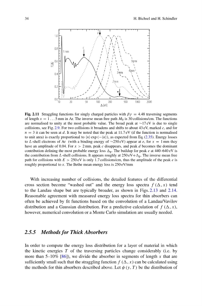
Fig. 2.11 Straggling functions for singly charged particles with βγ = 4.48 traversing segments
of length x = 1 . . . 5 mm in Ar. The inverse mean free path M 0 is 30 collisions/cm. The functions
are normalised to unity at the most probable value. The broad peak at ∼17 eV is due to single
collisions, see Fig. 2.9. For two collisions it broadens and shifts to about 43 eV, marked c, and for
n = 3 it can be seen at d. It may be noted that the peak at 11.7 eV (if the function is normalised
to unit area) is exactly proportional to n exp (−−n), as expected from Eq. (2.35). Energy losses
to L-shell electrons of Ar (with a binding energy of ∼250 eV) appear at e, for x = 1 mm they
have an amplitude of 0.04. For x > 2 mm, peak c disappears, and peak d becomes the dominant
contribution defining the most probable energy loss p . The buildup for peak e at 440–640 eV is
the contribution from L-shell collisions. It appears roughly at 250 eV+ p . The inverse mean free
path for collisions with E > 250 eV is only 1.7 collisions/cm, thus the amplitude of the peak e is
roughly proportional to x. The Bethe mean energy loss is 250 eV/mm
With increasing number of collisions, the detailed features of the differential
cross section become “washed out” and the energy loss spectra f (, x) tend
to the Landau shape but are typically broader, as shown in Figs. 2.13 and 2.14.
Reasonable agreement with measured energy loss spectra for thin absorbers can
often be achieved by fit functions based on the convolution of a Landau/Vavilov
distribution and a Gaussian distribution. For a predictive calculation of f (, x),
however, numerical convolution or a Monte Carlo simulation are usually needed.
2.5.5 Methods for Thick Absorbers
In order to compute the energy loss distribution for a layer of material in which
the kinetic energies T of the traversing particles change considerably (i.e. by
more than 5–10% [86]), we divide the absorber in segments of length x that are
sufficiently small such that the straggling function f (, x) can be calculated using
the methods for thin absorbers described above. Let φ (y, T ) be the distribution of
H. Bichsel and H. Schindler
Δ [eV]
f [Δ]
1 mm
2 mm
1.0
0.8
0.6
0.4
0.2
0.0
10
20
50
100
200
500
1000
2000
3 mm
4 mm
5 mm
c
d
Fig. 2.11 Straggling functions for singly charged particles with βγ = 4.48 traversing segments
of length x = 1 . . . 5 mm in Ar. The inverse mean free path M 0 is 30 collisions/cm. The functions
are normalised to unity at the most probable value. The broad peak at ∼17 eV is due to single
collisions, see Fig. 2.9. For two collisions it broadens and shifts to about 43 eV, marked c, and for
n = 3 it can be seen at d. It may be noted that the peak at 11.7 eV (if the function is normalised
to unit area) is exactly proportional to n exp (−−n), as expected from Eq. (2.35). Energy losses
to L-shell electrons of Ar (with a binding energy of ∼250 eV) appear at e, for x = 1 mm they
have an amplitude of 0.04. For x > 2 mm, peak c disappears, and peak d becomes the dominant
contribution defining the most probable energy loss p . The buildup for peak e at 440–640 eV is
the contribution from L-shell collisions. It appears roughly at 250 eV+ p . The inverse mean free
path for collisions with E > 250 eV is only 1.7 collisions/cm, thus the amplitude of the peak e is
roughly proportional to x. The Bethe mean energy loss is 250 eV/mm
With increasing number of collisions, the detailed features of the differential
cross section become “washed out” and the energy loss spectra f (, x) tend
to the Landau shape but are typically broader, as shown in Figs. 2.13 and 2.14.
Reasonable agreement with measured energy loss spectra for thin absorbers can
often be achieved by fit functions based on the convolution of a Landau/Vavilov
distribution and a Gaussian distribution. For a predictive calculation of f (, x),
however, numerical convolution or a Monte Carlo simulation are usually needed.
2.5.5 Methods for Thick Absorbers
In order to compute the energy loss distribution for a layer of material in which
the kinetic energies T of the traversing particles change considerably (i.e. by
more than 5–10% [86]), we divide the absorber in segments of length x that are
sufficiently small such that the straggling function f (, x) can be calculated using
the methods for thin absorbers described above. Let φ (y, T ) be the distribution of