

2 The Interaction of Radiation with Matter
33
where κ = ξ/E max . The full width at half maximum (FWHM) of the Landau
distribution 4 (2.37) is approximately 4.02ξ .
A somewhat unsatisfactory aspect of φ L (λ) is that its mean is undefined (a consequence of allowing arbitrarily large energy transfers E > E max ). This deficiency
was overcome by Vavilov [77] who, taking account of the kinematically allowed
maximum energy transfer E max and using the differential cross section (2.11) in I 2 ,
obtained
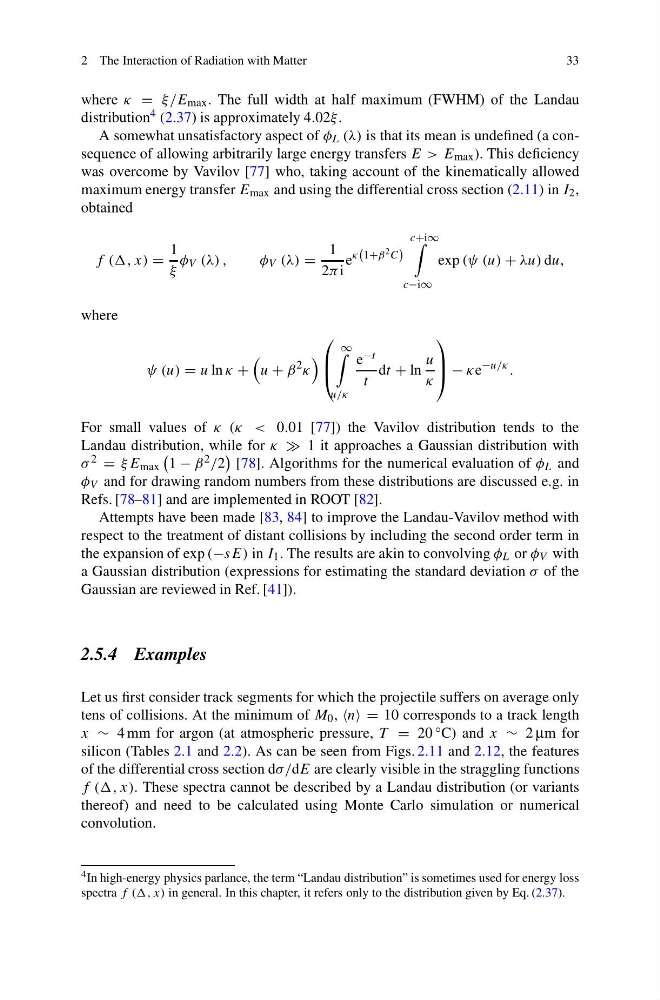
f (, x) =
1
ξ
φ V (λ) ,
φ V (λ) =
1
2πi
e
κ
1+β 2 C
c+i∞
c−i∞
exp (ψ (u) + λu) du,
where
ψ (u) = u ln κ +
u + β
2 κ
⎛
⎜
⎝
∞
u/κ
e −t
t
dt + ln
u
κ
⎞
⎟
⎠ − κe
−u/κ .
For small values of κ (κ < 0.01 [77]) the Vavilov distribution tends to the
Landau distribution, while for κ 1 it approaches a Gaussian distribution with
σ 2 = ξE max
1 − β 2 /2
[78]. Algorithms for the numerical evaluation of φ L and
φ V and for drawing random numbers from these distributions are discussed e.g. in
Refs. [78–81] and are implemented in ROOT [82].
Attempts have been made [83, 84] to improve the Landau-Vavilov method with
respect to the treatment of distant collisions by including the second order term in
the expansion of exp (−sE) in I 1 . The results are akin to convolving φ L or φ V with
a Gaussian distribution (expressions for estimating the standard deviation σ of the
Gaussian are reviewed in Ref. [41]).
2.5.4 Examples
Let us first consider track segments for which the projectile suffers on average only
tens of collisions. At the minimum of M 0 , = 10 corresponds to a track length
x ∼ 4 mm for argon (at atmospheric pressure, T = 20 ◦ C) and x ∼ 2 μm for
silicon (Tables 2.1 and 2.2). As can be seen from Figs. 2.11 and 2.12, the features
of the differential cross section dσ/dE are clearly visible in the straggling functions
f (, x). These spectra cannot be described by a Landau distribution (or variants
thereof) and need to be calculated using Monte Carlo simulation or numerical
convolution.
4 In high-energy physics parlance, the term “Landau distribution” is sometimes used for energy loss
spectra f ((, x) in general. In this chapter, it refers only to the distribution given by Eq. (2.37).
33
where κ = ξ/E max . The full width at half maximum (FWHM) of the Landau
distribution 4 (2.37) is approximately 4.02ξ .
A somewhat unsatisfactory aspect of φ L (λ) is that its mean is undefined (a consequence of allowing arbitrarily large energy transfers E > E max ). This deficiency
was overcome by Vavilov [77] who, taking account of the kinematically allowed
maximum energy transfer E max and using the differential cross section (2.11) in I 2 ,
obtained
f (, x) =
1
ξ
φ V (λ) ,
φ V (λ) =
1
2πi
e
κ
1+β 2 C
c+i∞
c−i∞
exp (ψ (u) + λu) du,
where
ψ (u) = u ln κ +
u + β
2 κ
⎛
⎜
⎝
∞
u/κ
e −t
t
dt + ln
u
κ
⎞
⎟
⎠ − κe
−u/κ .
For small values of κ (κ < 0.01 [77]) the Vavilov distribution tends to the
Landau distribution, while for κ 1 it approaches a Gaussian distribution with
σ 2 = ξE max
1 − β 2 /2
[78]. Algorithms for the numerical evaluation of φ L and
φ V and for drawing random numbers from these distributions are discussed e.g. in
Refs. [78–81] and are implemented in ROOT [82].
Attempts have been made [83, 84] to improve the Landau-Vavilov method with
respect to the treatment of distant collisions by including the second order term in
the expansion of exp (−sE) in I 1 . The results are akin to convolving φ L or φ V with
a Gaussian distribution (expressions for estimating the standard deviation σ of the
Gaussian are reviewed in Ref. [41]).
2.5.4 Examples
Let us first consider track segments for which the projectile suffers on average only
tens of collisions. At the minimum of M 0 , = 10 corresponds to a track length
x ∼ 4 mm for argon (at atmospheric pressure, T = 20 ◦ C) and x ∼ 2 μm for
silicon (Tables 2.1 and 2.2). As can be seen from Figs. 2.11 and 2.12, the features
of the differential cross section dσ/dE are clearly visible in the straggling functions
f (, x). These spectra cannot be described by a Landau distribution (or variants
thereof) and need to be calculated using Monte Carlo simulation or numerical
convolution.
4 In high-energy physics parlance, the term “Landau distribution” is sometimes used for energy loss
spectra f ((, x) in general. In this chapter, it refers only to the distribution given by Eq. (2.37).