

28
H. Bichsel and H. Schindler
differential cross section,
f
(1) (E) =
1
M 0
N
dσ
dE
,
and the probability distribution for a total energy loss in n collisions is obtained
from n-fold convolution of f (1) ,
f
(n) () =
f
(1)
⊗ f
(1)
⊗ · · · ⊗ f
(1)
n times
() =
dE f
(n−1) ( − E) f
(1) (E) ,
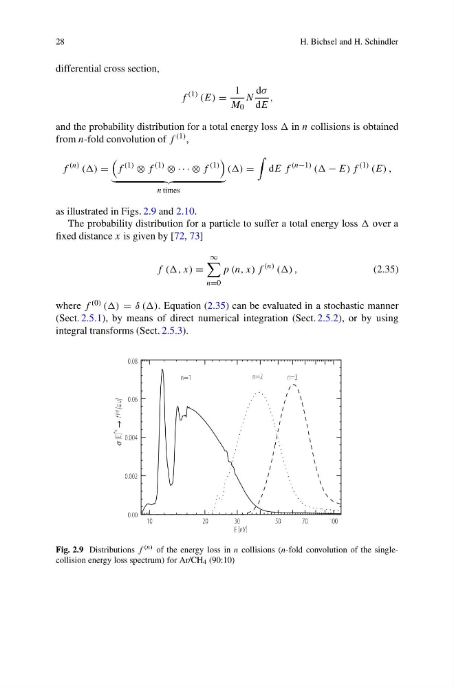
as illustrated in Figs. 2.9 and 2.10.
The probability distribution for a particle to suffer a total energy loss over a
fixed distance x is given by [72, 73]
f (, x) =
∞
n=0
p (n, x) f
(n) () ,
(2.35)
where f (0) () = δ (). Equation (2.35) can be evaluated in a stochastic manner
(Sect. 2.5.1), by means of direct numerical integration (Sect. 2.5.2), or by using
integral transforms (Sect. 2.5.3).
s [E] ù f (n)
[a.u]
*n
E [eV]
n=1
n=2
n=3
0.08
0.06
0.004
0.002
0.00
10
20
30
50
70
100
Fig. 2.9 Distributions f (n) of the energy loss in n collisions (n-fold convolution of the singlecollision energy loss spectrum) for Ar/CH 4 (90:10)
H. Bichsel and H. Schindler
differential cross section,
f
(1) (E) =
1
M 0
N
dσ
dE
,
and the probability distribution for a total energy loss in n collisions is obtained
from n-fold convolution of f (1) ,
f
(n) () =
f
(1)
⊗ f
(1)
⊗ · · · ⊗ f
(1)
n times
() =
dE f
(n−1) ( − E) f
(1) (E) ,
as illustrated in Figs. 2.9 and 2.10.
The probability distribution for a particle to suffer a total energy loss over a
fixed distance x is given by [72, 73]
f (, x) =
∞
n=0
p (n, x) f
(n) () ,
(2.35)
where f (0) () = δ (). Equation (2.35) can be evaluated in a stochastic manner
(Sect. 2.5.1), by means of direct numerical integration (Sect. 2.5.2), or by using
integral transforms (Sect. 2.5.3).
s [E] ù f (n)
[a.u]
*n
E [eV]
n=1
n=2
n=3
0.08
0.06
0.004
0.002
0.00
10
20
30
50
70
100
Fig. 2.9 Distributions f (n) of the energy loss in n collisions (n-fold convolution of the singlecollision energy loss spectrum) for Ar/CH 4 (90:10)