

2 The Interaction of Radiation with Matter
23
1
10
2
10
3
10
γ
β
10
]
-1
m
μ
[
0
M
1
10
2
10
3
10
γ
β
1
m]
μ
[keV/
1
M
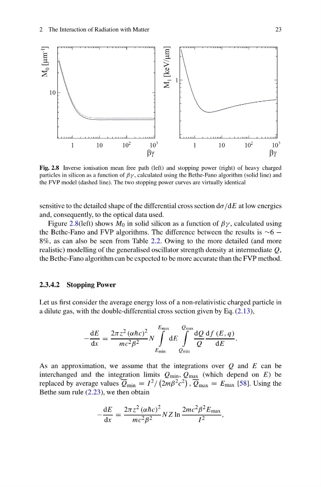
Fig. 2.8 Inverse ionisation mean free path (left) and stopping power (right) of heavy charged
particles in silicon as a function of βγ , calculated using the Bethe-Fano algorithm (solid line) and
the FVP model (dashed line). The two stopping power curves are virtually identical
sensitive to the detailed shape of the differential cross section dσ/dE at low energies
and, consequently, to the optical data used.
Figure 2.8(left) shows M 0 in solid silicon as a function of βγ , calculated using
the Bethe-Fano and FVP algorithms. The difference between the results is ∼6 −
8%, as can also be seen from Table 2.2. Owing to the more detailed (and more
realistic) modelling of the generalised oscillator strength density at intermediate Q,
the Bethe-Fano algorithm can be expected to be more accurate than the FVP method.
2.3.4.2 Stopping Power
Let us first consider the average energy loss of a non-relativistic charged particle in
a dilute gas, with the double-differential cross section given by Eq. (2.13),
−
dE
dx
=
2πz 2 (α ¯
hc)
2
mc 2 β 2 N
E max
E min
dE
Q max
Q min
dQ
Q
df (E, q)
dE
.
As an approximation, we assume that the integrations over Q and E can be
interchanged and the integration limits Q min , Q max (which depend on E) be
replaced by average values Q min = I 2 /
2mβ 2 c 2
, Q max = E max [58]. Using the
Bethe sum rule (2.23), we then obtain
−
dE
dx
=
2πz 2 (α ¯
hc)
2
mc 2 β 2 NZ ln
2mc 2 β 2 E max
I 2
,
23
1
10
2
10
3
10
γ
β
10
]
-1
m
μ
[
0
M
1
10
2
10
3
10
γ
β
1
m]
μ
[keV/
1
M
Fig. 2.8 Inverse ionisation mean free path (left) and stopping power (right) of heavy charged
particles in silicon as a function of βγ , calculated using the Bethe-Fano algorithm (solid line) and
the FVP model (dashed line). The two stopping power curves are virtually identical
sensitive to the detailed shape of the differential cross section dσ/dE at low energies
and, consequently, to the optical data used.
Figure 2.8(left) shows M 0 in solid silicon as a function of βγ , calculated using
the Bethe-Fano and FVP algorithms. The difference between the results is ∼6 −
8%, as can also be seen from Table 2.2. Owing to the more detailed (and more
realistic) modelling of the generalised oscillator strength density at intermediate Q,
the Bethe-Fano algorithm can be expected to be more accurate than the FVP method.
2.3.4.2 Stopping Power
Let us first consider the average energy loss of a non-relativistic charged particle in
a dilute gas, with the double-differential cross section given by Eq. (2.13),
−
dE
dx
=
2πz 2 (α ¯
hc)
2
mc 2 β 2 N
E max
E min
dE
Q max
Q min
dQ
Q
df (E, q)
dE
.
As an approximation, we assume that the integrations over Q and E can be
interchanged and the integration limits Q min , Q max (which depend on E) be
replaced by average values Q min = I 2 /
2mβ 2 c 2
, Q max = E max [58]. Using the
Bethe sum rule (2.23), we then obtain
−
dE
dx
=
2πz 2 (α ¯
hc)
2
mc 2 β 2 NZ ln
2mc 2 β 2 E max
I 2
,