

6 Calorimetry
211
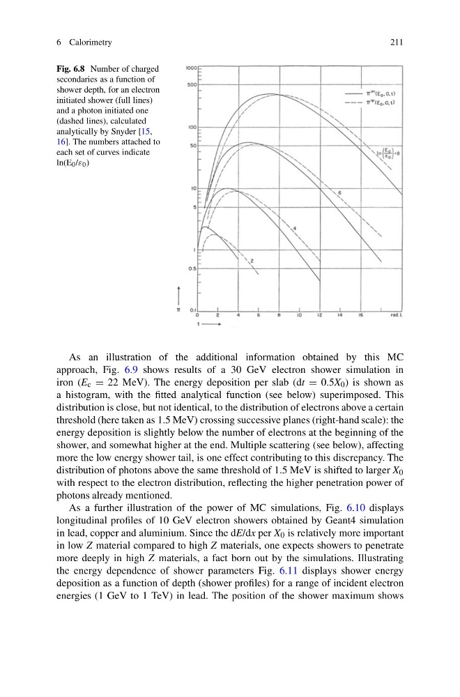
Fig. 6.8 Number of charged
secondaries as a function of
shower depth, for an electron
initiated shower (full lines)
and a photon initiated one
(dashed lines), calculated
analytically by Snyder [15,
16]. The numbers attached to
each set of curves indicate
ln(E 0 /ε 0 )
As an illustration of the additional information obtained by this MC
approach, Fig. 6.9 shows results of a 30 GeV electron shower simulation in
iron (E c = 22 MeV). The energy deposition per slab (dt = 0.5X 0 ) is shown as
a histogram, with the fitted analytical function (see below) superimposed. This
distribution is close, but not identical, to the distribution of electrons above a certain
threshold (here taken as 1.5 MeV) crossing successive planes (right-hand scale): the
energy deposition is slightly below the number of electrons at the beginning of the
shower, and somewhat higher at the end. Multiple scattering (see below), affecting
more the low energy shower tail, is one effect contributing to this discrepancy. The
distribution of photons above the same threshold of 1.5 MeV is shifted to larger X 0
with respect to the electron distribution, reflecting the higher penetration power of
photons already mentioned.
As a further illustration of the power of MC simulations, Fig. 6.10 displays
longitudinal profiles of 10 GeV electron showers obtained by Geant4 simulation
in lead, copper and aluminium. Since the dE/dx per X 0 is relatively more important
in low Z material compared to high Z materials, one expects showers to penetrate
more deeply in high Z materials, a fact born out by the simulations. Illustrating
the energy dependence of shower parameters Fig. 6.11 displays shower energy
deposition as a function of depth (shower profiles) for a range of incident electron
energies (1 GeV to 1 TeV) in lead. The position of the shower maximum shows
211
Fig. 6.8 Number of charged
secondaries as a function of
shower depth, for an electron
initiated shower (full lines)
and a photon initiated one
(dashed lines), calculated
analytically by Snyder [15,
16]. The numbers attached to
each set of curves indicate
ln(E 0 /ε 0 )
As an illustration of the additional information obtained by this MC
approach, Fig. 6.9 shows results of a 30 GeV electron shower simulation in
iron (E c = 22 MeV). The energy deposition per slab (dt = 0.5X 0 ) is shown as
a histogram, with the fitted analytical function (see below) superimposed. This
distribution is close, but not identical, to the distribution of electrons above a certain
threshold (here taken as 1.5 MeV) crossing successive planes (right-hand scale): the
energy deposition is slightly below the number of electrons at the beginning of the
shower, and somewhat higher at the end. Multiple scattering (see below), affecting
more the low energy shower tail, is one effect contributing to this discrepancy. The
distribution of photons above the same threshold of 1.5 MeV is shifted to larger X 0
with respect to the electron distribution, reflecting the higher penetration power of
photons already mentioned.
As a further illustration of the power of MC simulations, Fig. 6.10 displays
longitudinal profiles of 10 GeV electron showers obtained by Geant4 simulation
in lead, copper and aluminium. Since the dE/dx per X 0 is relatively more important
in low Z material compared to high Z materials, one expects showers to penetrate
more deeply in high Z materials, a fact born out by the simulations. Illustrating
the energy dependence of shower parameters Fig. 6.11 displays shower energy
deposition as a function of depth (shower profiles) for a range of incident electron
energies (1 GeV to 1 TeV) in lead. The position of the shower maximum shows