

86
W. Herr and E. Forest
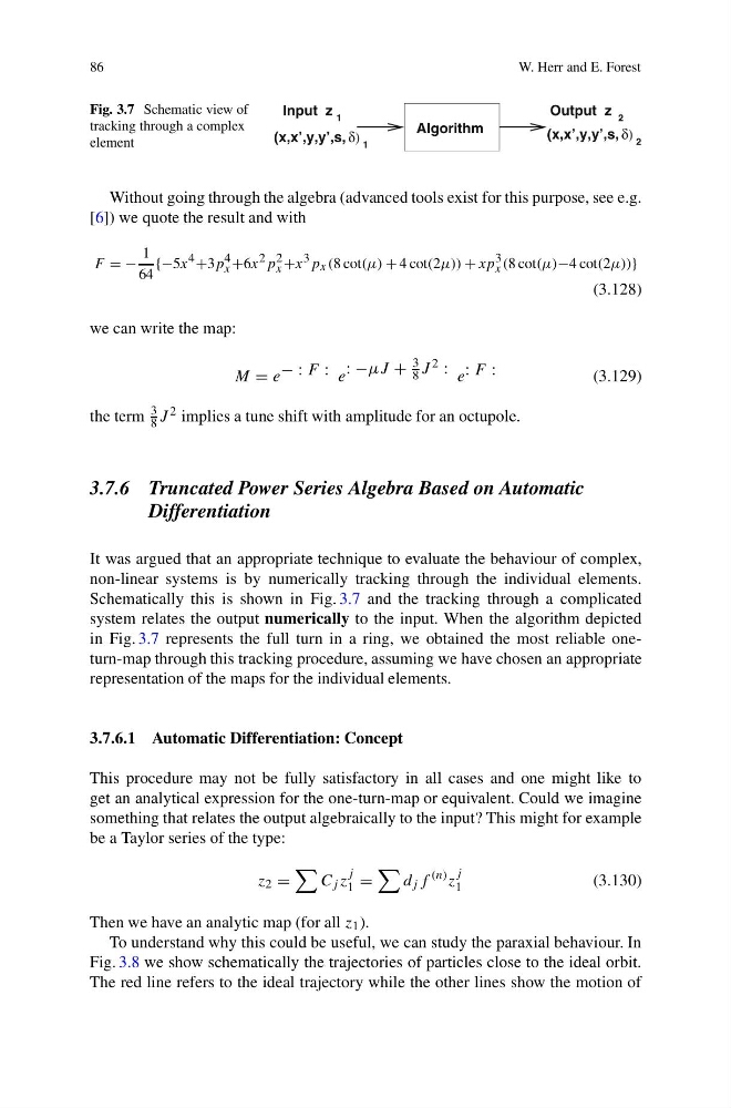
Fig. 3.7 Schematic view of
tracking through a complex
element
(x,x’,y,y’,s, δ)
(x,x’,y,y’,s, δ)
Algorithm
1
2
2
1
Output z
Input z
Without going through the algebra (advanced tools exist for this purpose, see e.g.
[6]) we quote the result and with
F = −
1
64
{−5x 4 +3p 4
x +6x 2 p 2
x +x 3 p x (8 cot(μ) + 4 cot(2μ)) + xp 3
x (8 cot(μ)−4 cot(2μ))}
(3.128)
we can write the map:
M = e − : F : e : −μJ +
3
8 J 2 : e : F :
(3.129)
the term
3
8 J 2 implies a tune shift with amplitude for an octupole.
3.7.6 Truncated Power Series Algebra Based on Automatic
Differentiation
It was argued that an appropriate technique to evaluate the behaviour of complex,
non-linear systems is by numerically tracking through the individual elements.
Schematically this is shown in Fig. 3.7 and the tracking through a complicated
system relates the output numerically to the input. When the algorithm depicted
in Fig. 3.7 represents the full turn in a ring, we obtained the most reliable oneturn-map through this tracking procedure, assuming we have chosen an appropriate
representation of the maps for the individual elements.
3.7.6.1 Automatic Differentiation: Concept
This procedure may not be fully satisfactory in all cases and one might like to
get an analytical expression for the one-turn-map or equivalent. Could we imagine
something that relates the output algebraically to the input? This might for example
be a Taylor series of the type:
z 2 =
C j z
j
1 =
d j f
(n) z
j
1
(3.130)
Then we have an analytic map (for all z 1 ).
To understand why this could be useful, we can study the paraxial behaviour. In
Fig. 3.8 we show schematically the trajectories of particles close to the ideal orbit.
The red line refers to the ideal trajectory while the other lines show the motion of
W. Herr and E. Forest
Fig. 3.7 Schematic view of
tracking through a complex
element
(x,x’,y,y’,s, δ)
(x,x’,y,y’,s, δ)
Algorithm
1
2
2
1
Output z
Input z
Without going through the algebra (advanced tools exist for this purpose, see e.g.
[6]) we quote the result and with
F = −
1
64
{−5x 4 +3p 4
x +6x 2 p 2
x +x 3 p x (8 cot(μ) + 4 cot(2μ)) + xp 3
x (8 cot(μ)−4 cot(2μ))}
(3.128)
we can write the map:
M = e − : F : e : −μJ +
3
8 J 2 : e : F :
(3.129)
the term
3
8 J 2 implies a tune shift with amplitude for an octupole.
3.7.6 Truncated Power Series Algebra Based on Automatic
Differentiation
It was argued that an appropriate technique to evaluate the behaviour of complex,
non-linear systems is by numerically tracking through the individual elements.
Schematically this is shown in Fig. 3.7 and the tracking through a complicated
system relates the output numerically to the input. When the algorithm depicted
in Fig. 3.7 represents the full turn in a ring, we obtained the most reliable oneturn-map through this tracking procedure, assuming we have chosen an appropriate
representation of the maps for the individual elements.
3.7.6.1 Automatic Differentiation: Concept
This procedure may not be fully satisfactory in all cases and one might like to
get an analytical expression for the one-turn-map or equivalent. Could we imagine
something that relates the output algebraically to the input? This might for example
be a Taylor series of the type:
z 2 =
C j z
j
1 =
d j f
(n) z
j
1
(3.130)
Then we have an analytic map (for all z 1 ).
To understand why this could be useful, we can study the paraxial behaviour. In
Fig. 3.8 we show schematically the trajectories of particles close to the ideal orbit.
The red line refers to the ideal trajectory while the other lines show the motion of