692
M. Dohlus et al.
Third Order Equation
The main physics of the high-gain FEL is contained in the first-order Eq. (11.77) but
these can only be solved numerically. If the modulation current ˜
j 1 remains small a
linear third order differential equation for the electric field can be derived (see e.g.
[7, 14, 20, 21]):
˜
E
x + 4ik u η ˜
E
x − 4k
2
u η
2 ˜
E
x −
i
√
3L g0
3
˜
E x = 0
(11.78)
with the 1D power gain length
L g0 =
1
√
3
4γ 3
r m e
μ 0 ˆ
K 2 e 2 k u n e
1/3
.
(11.79)
Exponential Gain and Saturation
The solution of Eq. (11.78) is of the form ˜
E x (z) =
3
j =1 A j exp
α j z
. For
the special case η = 0 (electrons are on resonance energy) one finds α 1,2 =
±1 + i/
√
3
/
2L g0
, α 3 = −i/
√
3L g0
. In case of laser seeding (see below)
with an initial field E 0 , all amplitudes are equal, A j = E 0 /3. The light power
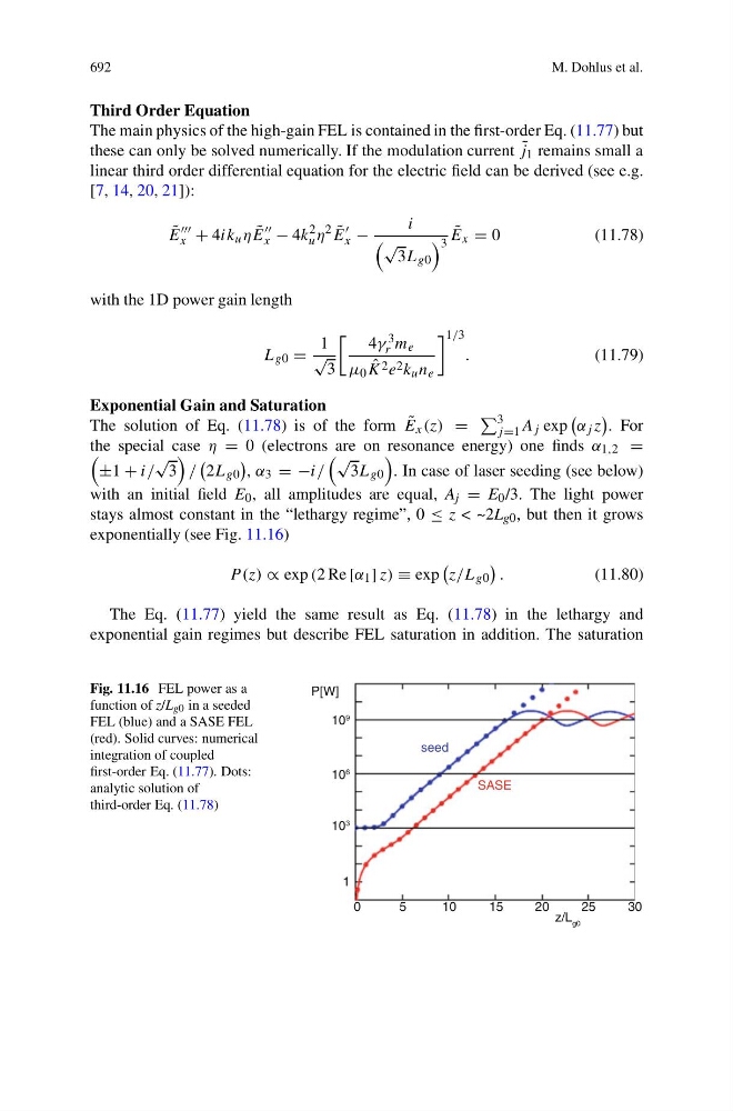
stays almost constant in the “lethargy regime”, 0 ≤ z < ~2L g0 , but then it grows
exponentially (see Fig. 11.16)
P (z) ∝ exp (2 Re [α 1 ] z) ≡ exp
z/L g0
.
(11.80)
The Eq. (11.77) yield the same result as Eq. (11.78) in the lethargy and
exponential gain regimes but describe FEL saturation in addition. The saturation
Fig. 11.16 FEL power as a
function of z/L g0 in a seeded
FEL (blue) and a SASE FEL
(red). Solid curves: numerical
integration of coupled
first-order Eq. (11.77). Dots:
analytic solution of
third-order Eq. (11.78)
P[W]
seed
SASE
10
9
10
3
1
0
5
10
15
20
25
30
z/L g0
10
6