

11 Application of Accelerators and Storage Rings
665
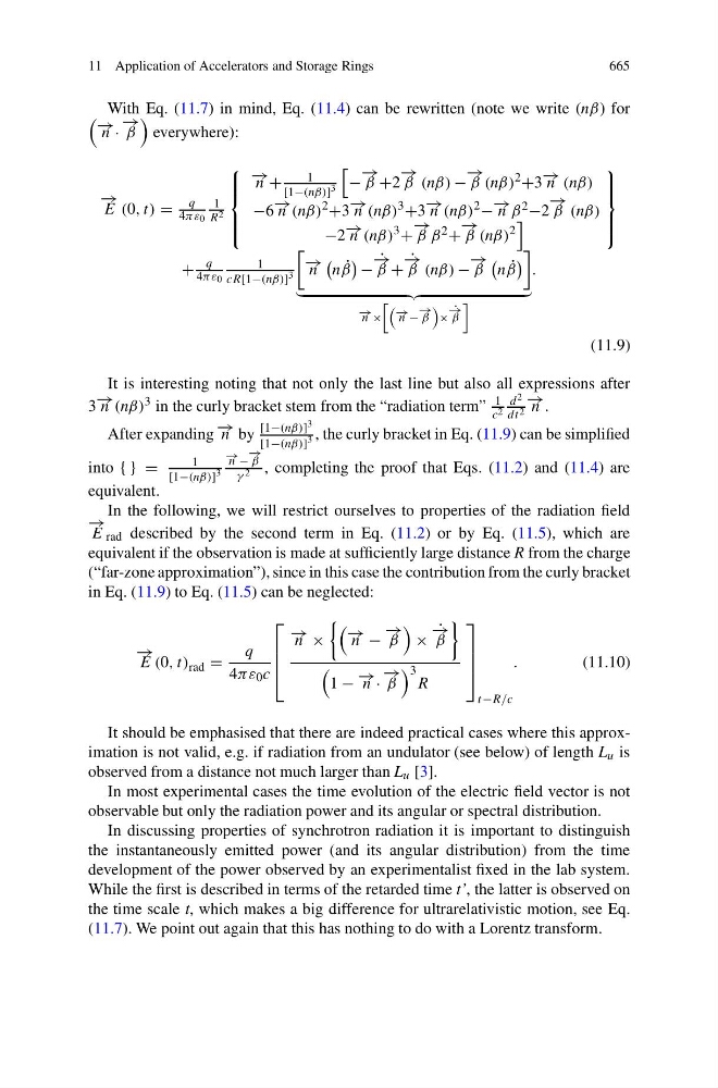
With Eq. (11.7) in mind, Eq. (11.4) can be rewritten (note we write (nβ) for
− → n ·
− →
β
everywhere):
− →
E (0, t) =
q
4πε 0
1
R 2
⎧
⎪ ⎪ ⎨
⎪ ⎪ ⎩
− → n +
1
[1−(nβ)] 3
−
− →
β +2
− →
β (nβ) −
− →
β (nβ)
2
+3 − → n (nβ)
−6 − → n (nβ)
2
+3 − → n (nβ)
3
+3 − → n (nβ)
2
− − → n β 2 −2
− →
β (nβ)
−2 − → n (nβ)
3
+
− →
β β 2 +
− →
β (nβ)
2
⎫
⎪ ⎪ ⎬
⎪ ⎪ ⎭
+
q
4πε 0
1
cR[1−(nβ)] 3
− → n
n ˙
β
−
˙
− →
β +
˙
− →
β (nβ) −
− →
β
n ˙
β
− → n ×
− → n −
− →
β
×
˙
− →
β
.
(11.9)
It is interesting noting that not only the last line but also all expressions after
3 − → n (nβ) 3 in the curly bracket stem from the “radiation term”
1
c 2
d 2
dt 2
− → n .
After expanding − → n by
[1−(nβ)] 3
[1−(nβ)] 3 , the curly bracket in Eq. (11.9) can be simplified
into { } =
1
[1−(nβ)] 3
− → n −
− →
β
γ 2 , completing the proof that Eqs. (11.2) and (11.4) are
equivalent.
In the following, we will restrict ourselves to properties of the radiation field
− →
E rad described by the second term in Eq. (11.2) or by Eq. (11.5), which are
equivalent if the observation is made at sufficiently large distance R from the charge
(“far-zone approximation”), since in this case the contribution from the curly bracket
in Eq. (11.9) to Eq. (11.5) can be neglected:
− →
E (0, t) rad =
q
4πε 0 c
⎡
⎢
⎢
⎣
− → n ×
− → n −
− →
β
×
˙
− →
β
1 − − → n ·
− →
β
3
R
⎤
⎥
⎥
⎦
t −R/c
.
(11.10)
It should be emphasised that there are indeed practical cases where this approximation is not valid, e.g. if radiation from an undulator (see below) of length L u is
observed from a distance not much larger than L u [3].
In most experimental cases the time evolution of the electric field vector is not
observable but only the radiation power and its angular or spectral distribution.
In discussing properties of synchrotron radiation it is important to distinguish
the instantaneously emitted power (and its angular distribution) from the time
development of the power observed by an experimentalist fixed in the lab system.
While the first is described in terms of the retarded time t’, the latter is observed on
the time scale t, which makes a big difference for ultrarelativistic motion, see Eq.
(11.7). We point out again that this has nothing to do with a Lorentz transform.