

534
M. Lamont et al.
9.4.1.1 First and Second Order Example
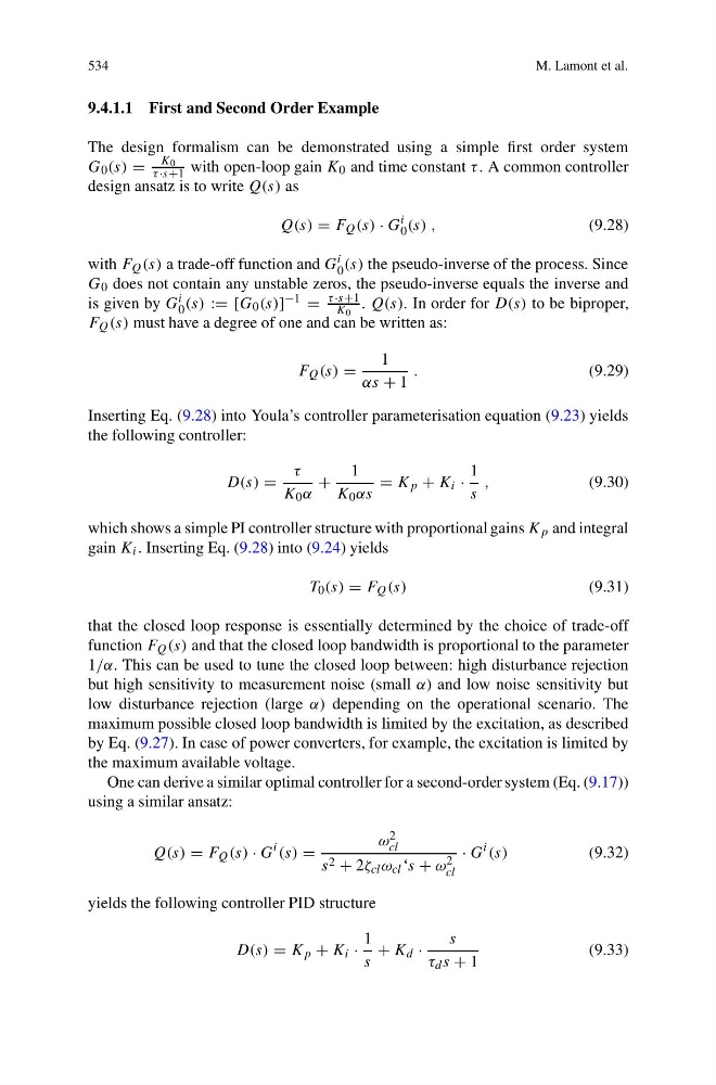
The design formalism can be demonstrated using a simple first order system
G 0 (s) =
K 0
τ ·s+1 with open-loop gain K 0 and time constant τ . A common controller
design ansatz is to write Q(s) as
Q(s) = F Q (s) · G
i
0 (s) ,
(9.28)
with F Q (s) a trade-off function and G
i
0 (s) the pseudo-inverse of the process. Since
G 0 does not contain any unstable zeros, the pseudo-inverse equals the inverse and
is given by G
i
0 (s) := [G 0 (s)] −1 =
τ ·s+1
K 0
. Q(s). In order for D(s) to be biproper,
F Q (s) must have a degree of one and can be written as:
F Q (s) =
1
αs + 1
.
(9.29)
Inserting Eq. (9.28) into Youla’s controller parameterisation equation (9.23) yields
the following controller:
D(s) =
τ
K 0 α
+
1
K 0 αs
= K p + K i ·
1
s
,
(9.30)
which shows a simple PI controller structure with proportional gains K p and integral
gain K i . Inserting Eq. (9.28) into (9.24) yields
T 0 (s) = F Q (s)
(9.31)
that the closed loop response is essentially determined by the choice of trade-off
function F Q (s) and that the closed loop bandwidth is proportional to the parameter
1/α. This can be used to tune the closed loop between: high disturbance rejection
but high sensitivity to measurement noise (small α) and low noise sensitivity but
low disturbance rejection (large α) depending on the operational scenario. The
maximum possible closed loop bandwidth is limited by the excitation, as described
by Eq. (9.27). In case of power converters, for example, the excitation is limited by
the maximum available voltage.
One can derive a similar optimal controller for a second-order system (Eq. (9.17))
using a similar ansatz:
Q(s) = F Q (s) · G
i (s) =
ω 2
cl
s 2 + 2ζ cl ω cl ‘s + ω 2
cl
· G
i (s)
(9.32)
yields the following controller PID structure
D(s) = K p + K i ·
1
s
+ K d ·
s
τ d s + 1
(9.33)
M. Lamont et al.
9.4.1.1 First and Second Order Example
The design formalism can be demonstrated using a simple first order system
G 0 (s) =
K 0
τ ·s+1 with open-loop gain K 0 and time constant τ . A common controller
design ansatz is to write Q(s) as
Q(s) = F Q (s) · G
i
0 (s) ,
(9.28)
with F Q (s) a trade-off function and G
i
0 (s) the pseudo-inverse of the process. Since
G 0 does not contain any unstable zeros, the pseudo-inverse equals the inverse and
is given by G
i
0 (s) := [G 0 (s)] −1 =
τ ·s+1
K 0
. Q(s). In order for D(s) to be biproper,
F Q (s) must have a degree of one and can be written as:
F Q (s) =
1
αs + 1
.
(9.29)
Inserting Eq. (9.28) into Youla’s controller parameterisation equation (9.23) yields
the following controller:
D(s) =
τ
K 0 α
+
1
K 0 αs
= K p + K i ·
1
s
,
(9.30)
which shows a simple PI controller structure with proportional gains K p and integral
gain K i . Inserting Eq. (9.28) into (9.24) yields
T 0 (s) = F Q (s)
(9.31)
that the closed loop response is essentially determined by the choice of trade-off
function F Q (s) and that the closed loop bandwidth is proportional to the parameter
1/α. This can be used to tune the closed loop between: high disturbance rejection
but high sensitivity to measurement noise (small α) and low noise sensitivity but
low disturbance rejection (large α) depending on the operational scenario. The
maximum possible closed loop bandwidth is limited by the excitation, as described
by Eq. (9.27). In case of power converters, for example, the excitation is limited by
the maximum available voltage.
One can derive a similar optimal controller for a second-order system (Eq. (9.17))
using a similar ansatz:
Q(s) = F Q (s) · G
i (s) =
ω 2
cl
s 2 + 2ζ cl ω cl ‘s + ω 2
cl
· G
i (s)
(9.32)
yields the following controller PID structure
D(s) = K p + K i ·
1
s
+ K d ·
s
τ d s + 1
(9.33)