

7 Design and Principles of Linear Accelerators and Colliders
311
The distribution of accelerating gradient E acc (z) along the structure is obtained
by solving Eqs. (7.15 and 7.16) for a given input power P in . Integrating it over the
structure length L gives the overall structure energy gain:
V AS =
L
0
E acc (z)dz.
(7.17)
Then the steady-state RF-to-beam efficiency is defined as following:
η 0 =
V AS I
P in
.
(7.18)
For linacs operating in pulsed mode, the structure must be filled on each pulse
before beam is injected. Filling time of the structure is defined as
t f =
L
0
dz
v g (z)
.
(7.19)
In this case, RF-to-beam efficiency, η, is reduced by the ratio of the bunch train
length t b = N b /f b , where N b is the number of bunches and the RF pulse length
t p = t b + t f :
η = η 0
t b
t p
.
(7.20)
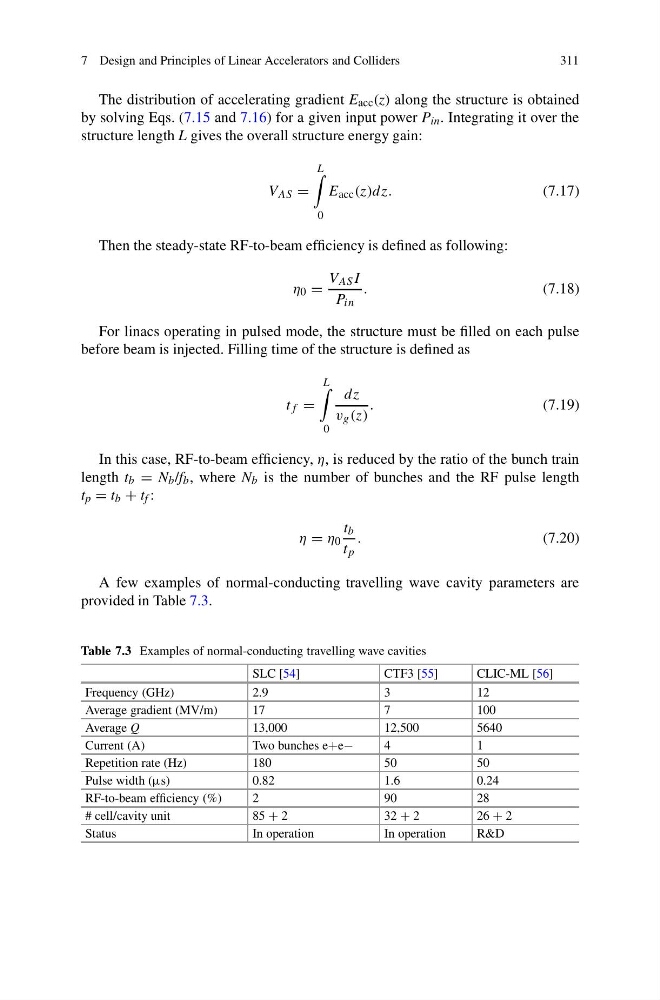
A few examples of normal-conducting travelling wave cavity parameters are
provided in Table 7.3.
Table 7.3 Examples of normal-conducting travelling wave cavities
SLC [54]
CTF3 [55]
CLIC-ML [56]
Frequency (GHz)
2.9
3
12
Average gradient (MV/m)
17
7
100
Average Q
13,000
12,500
5640
Current (A)
Two bunches e+e−
4
1
Repetition rate (Hz)
180
50
50
Pulse width (μs)
0.82
1.6
0.24
RF-to-beam efficiency (%)
2
90
28
# cell/cavity unit
85 + 2
32 + 2
26 + 2
Status
In operation
In operation
R&D
311
The distribution of accelerating gradient E acc (z) along the structure is obtained
by solving Eqs. (7.15 and 7.16) for a given input power P in . Integrating it over the
structure length L gives the overall structure energy gain:
V AS =
L
0
E acc (z)dz.
(7.17)
Then the steady-state RF-to-beam efficiency is defined as following:
η 0 =
V AS I
P in
.
(7.18)
For linacs operating in pulsed mode, the structure must be filled on each pulse
before beam is injected. Filling time of the structure is defined as
t f =
L
0
dz
v g (z)
.
(7.19)
In this case, RF-to-beam efficiency, η, is reduced by the ratio of the bunch train
length t b = N b /f b , where N b is the number of bunches and the RF pulse length
t p = t b + t f :
η = η 0
t b
t p
.
(7.20)
A few examples of normal-conducting travelling wave cavity parameters are
provided in Table 7.3.
Table 7.3 Examples of normal-conducting travelling wave cavities
SLC [54]
CTF3 [55]
CLIC-ML [56]
Frequency (GHz)
2.9
3
12
Average gradient (MV/m)
17
7
100
Average Q
13,000
12,500
5640
Current (A)
Two bunches e+e−
4
1
Repetition rate (Hz)
180
50
50
Pulse width (μs)
0.82
1.6
0.24
RF-to-beam efficiency (%)
2
90
28
# cell/cavity unit
85 + 2
32 + 2
26 + 2
Status
In operation
In operation
R&D