

4 Impedance and Collective Effects
133
Here, Q c is the coherent betatron tune to be determined, J x,y are the action variables in the horizontal and vertical plane respectively, with f (J x , J y ) the distribution
function, ΔQ x
coh is the horizontal coherent tune shift, Q x (J x , J y ) is the horizontal
tune in the presence of octupoles, m is the head–tail mode number, and Q s is the
small-amplitude synchrotron tune (the longitudinal spread is neglected).
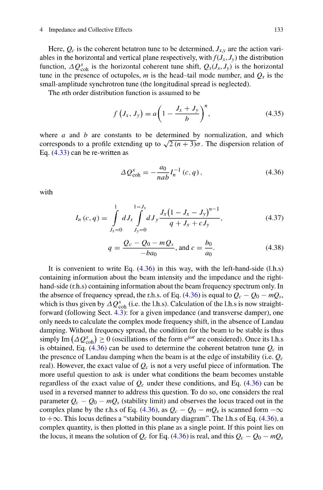
The nth order distribution function is assumed to be
f
J x , J y
= a
1 −
J x + J y
b
n
,
(4.35)
where a and b are constants to be determined by normalization, and which
corresponds to a profile extending up to
√
2 (n + 3)σ . The dispersion relation of
Eq. (4.33) can be re-written as
ΔQ
x
coh = −
a 0
nab
I
−1
n (c, q) ,
(4.36)
with
I n (c, q) =
1
J x =0
dJ x
1−J x
J y =0
dJ y
J x
1 − J x − J y
n−1
q + J x + cJ y
,
(4.37)
q =
Q c − Q 0 − mQ s
−ba 0
, and c =
b 0
a 0
.
(4.38)
It is convenient to write Eq. (4.36) in this way, with the left-hand-side (l.h.s)
containing information about the beam intensity and the impedance and the righthand-side (r.h.s) containing information about the beam frequency spectrum only. In
the absence of frequency spread, the r.h.s. of Eq. (4.36) is equal to Q c − Q 0 − mQ s ,
which is thus given by ΔQ
x
coh (i.e. the l.h.s). Calculation of the l.h.s is now straightforward (following Sect. 4.3): for a given impedance (and transverse damper), one
only needs to calculate the complex mode frequency shift, in the absence of Landau
damping. Without frequency spread, the condition for the beam to be stable is thus
simply Im
ΔQ
x
coh
≥ 0 (oscillations of the form e jωt are considered). Once its l.h.s
is obtained, Eq. (4.36) can be used to determine the coherent betatron tune Q c in
the presence of Landau damping when the beam is at the edge of instability (i.e. Q c
real). However, the exact value of Q c is not a very useful piece of information. The
more useful question to ask is under what conditions the beam becomes unstable
regardless of the exact value of Q c under these conditions, and Eq. (4.36) can be
used in a reversed manner to address this question. To do so, one considers the real
parameter Q c − Q 0 − mQ s (stability limit) and observes the locus traced out in the
complex plane by the r.h.s of Eq. (4.36), as Q c − Q 0 − mQ s is scanned form −∞
to +∞. This locus defines a “stability boundary diagram”. The l.h.s of Eq. (4.36), a
complex quantity, is then plotted in this plane as a single point. If this point lies on
the locus, it means the solution of Q c for Eq. (4.36) is real, and this Q c − Q 0 − mQ s
133
Here, Q c is the coherent betatron tune to be determined, J x,y are the action variables in the horizontal and vertical plane respectively, with f (J x , J y ) the distribution
function, ΔQ x
coh is the horizontal coherent tune shift, Q x (J x , J y ) is the horizontal
tune in the presence of octupoles, m is the head–tail mode number, and Q s is the
small-amplitude synchrotron tune (the longitudinal spread is neglected).
The nth order distribution function is assumed to be
f
J x , J y
= a
1 −
J x + J y
b
n
,
(4.35)
where a and b are constants to be determined by normalization, and which
corresponds to a profile extending up to
√
2 (n + 3)σ . The dispersion relation of
Eq. (4.33) can be re-written as
ΔQ
x
coh = −
a 0
nab
I
−1
n (c, q) ,
(4.36)
with
I n (c, q) =
1
J x =0
dJ x
1−J x
J y =0
dJ y
J x
1 − J x − J y
n−1
q + J x + cJ y
,
(4.37)
q =
Q c − Q 0 − mQ s
−ba 0
, and c =
b 0
a 0
.
(4.38)
It is convenient to write Eq. (4.36) in this way, with the left-hand-side (l.h.s)
containing information about the beam intensity and the impedance and the righthand-side (r.h.s) containing information about the beam frequency spectrum only. In
the absence of frequency spread, the r.h.s. of Eq. (4.36) is equal to Q c − Q 0 − mQ s ,
which is thus given by ΔQ
x
coh (i.e. the l.h.s). Calculation of the l.h.s is now straightforward (following Sect. 4.3): for a given impedance (and transverse damper), one
only needs to calculate the complex mode frequency shift, in the absence of Landau
damping. Without frequency spread, the condition for the beam to be stable is thus
simply Im
ΔQ
x
coh
≥ 0 (oscillations of the form e jωt are considered). Once its l.h.s
is obtained, Eq. (4.36) can be used to determine the coherent betatron tune Q c in
the presence of Landau damping when the beam is at the edge of instability (i.e. Q c
real). However, the exact value of Q c is not a very useful piece of information. The
more useful question to ask is under what conditions the beam becomes unstable
regardless of the exact value of Q c under these conditions, and Eq. (4.36) can be
used in a reversed manner to address this question. To do so, one considers the real
parameter Q c − Q 0 − mQ s (stability limit) and observes the locus traced out in the
complex plane by the r.h.s of Eq. (4.36), as Q c − Q 0 − mQ s is scanned form −∞
to +∞. This locus defines a “stability boundary diagram”. The l.h.s of Eq. (4.36), a
complex quantity, is then plotted in this plane as a single point. If this point lies on
the locus, it means the solution of Q c for Eq. (4.36) is real, and this Q c − Q 0 − mQ s