

114
E. Metral et al.
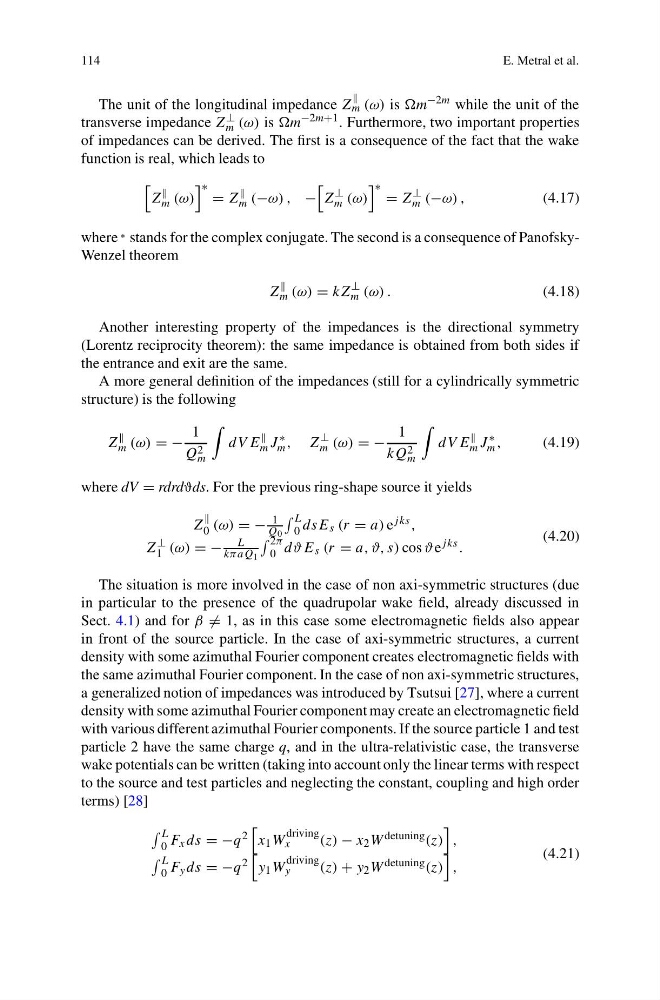
The unit of the longitudinal impedance Z
m (ω) is −2m while the unit of the
transverse impedance Z ⊥
m (ω) is −2m+1 . Furthermore, two important properties
of impedances can be derived. The first is a consequence of the fact that the wake
function is real, which leads to
Z
m (ω)
∗ = Z
m (−ω) , −
Z
⊥
m (ω)
∗ = Z
⊥
m (−ω) ,
(4.17)
where ∗ stands for the complex conjugate. The second is a consequence of PanofskyWenzel theorem
Z
m (ω) = kZ
⊥
m (ω) .
(4.18)
Another interesting property of the impedances is the directional symmetry
(Lorentz reciprocity theorem): the same impedance is obtained from both sides if
the entrance and exit are the same.
A more general definition of the impedances (still for a cylindrically symmetric
structure) is the following
Z
m (ω) = −
1
Q 2
m
dV E
m J
∗
m , Z
⊥
m (ω) = −
1
kQ 2
m
dV E
m J
∗
m ,
(4.19)
where dV = rdrdϑds. For the previous ring-shape source it yields
Z
0 (ω) = −
1
Q 0
L
0 dsE s (r = a) e jks ,
Z ⊥
1 (ω) = −
L
kπaQ 1
2π
0 dϑE s (r = a, ϑ, s) cos ϑe jks .
(4.20)
The situation is more involved in the case of non axi-symmetric structures (due
in particular to the presence of the quadrupolar wake field, already discussed in
Sect. 4.1) and for β = 1, as in this case some electromagnetic fields also appear
in front of the source particle. In the case of axi-symmetric structures, a current
density with some azimuthal Fourier component creates electromagnetic fields with
the same azimuthal Fourier component. In the case of non axi-symmetric structures,
a generalized notion of impedances was introduced by Tsutsui [27], where a current
density with some azimuthal Fourier component may create an electromagnetic field
with various different azimuthal Fourier components. If the source particle 1 and test
particle 2 have the same charge q, and in the ultra-relativistic case, the transverse
wake potentials can be written (taking into account only the linear terms with respect
to the source and test particles and neglecting the constant, coupling and high order
terms) [28]
L
0 F x ds = −q 2
x 1 W
driving
x
(z) − x 2 W detuning (z)
,
L
0 F y ds = −q 2
y 1 W
driving
y
(z) + y 2 W detuning (z)
,
(4.21)
E. Metral et al.
The unit of the longitudinal impedance Z
m (ω) is −2m while the unit of the
transverse impedance Z ⊥
m (ω) is −2m+1 . Furthermore, two important properties
of impedances can be derived. The first is a consequence of the fact that the wake
function is real, which leads to
Z
m (ω)
∗ = Z
m (−ω) , −
Z
⊥
m (ω)
∗ = Z
⊥
m (−ω) ,
(4.17)
where ∗ stands for the complex conjugate. The second is a consequence of PanofskyWenzel theorem
Z
m (ω) = kZ
⊥
m (ω) .
(4.18)
Another interesting property of the impedances is the directional symmetry
(Lorentz reciprocity theorem): the same impedance is obtained from both sides if
the entrance and exit are the same.
A more general definition of the impedances (still for a cylindrically symmetric
structure) is the following
Z
m (ω) = −
1
Q 2
m
dV E
m J
∗
m , Z
⊥
m (ω) = −
1
kQ 2
m
dV E
m J
∗
m ,
(4.19)
where dV = rdrdϑds. For the previous ring-shape source it yields
Z
0 (ω) = −
1
Q 0
L
0 dsE s (r = a) e jks ,
Z ⊥
1 (ω) = −
L
kπaQ 1
2π
0 dϑE s (r = a, ϑ, s) cos ϑe jks .
(4.20)
The situation is more involved in the case of non axi-symmetric structures (due
in particular to the presence of the quadrupolar wake field, already discussed in
Sect. 4.1) and for β = 1, as in this case some electromagnetic fields also appear
in front of the source particle. In the case of axi-symmetric structures, a current
density with some azimuthal Fourier component creates electromagnetic fields with
the same azimuthal Fourier component. In the case of non axi-symmetric structures,
a generalized notion of impedances was introduced by Tsutsui [27], where a current
density with some azimuthal Fourier component may create an electromagnetic field
with various different azimuthal Fourier components. If the source particle 1 and test
particle 2 have the same charge q, and in the ultra-relativistic case, the transverse
wake potentials can be written (taking into account only the linear terms with respect
to the source and test particles and neglecting the constant, coupling and high order
terms) [28]
L
0 F x ds = −q 2
x 1 W
driving
x
(z) − x 2 W detuning (z)
,
L
0 F y ds = −q 2
y 1 W
driving
y
(z) + y 2 W detuning (z)
,
(4.21)