

4 Impedance and Collective Effects
107
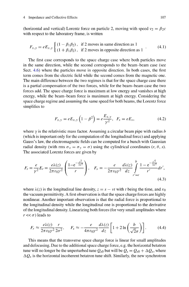
(horizontal and vertical) Lorentz force on particle 2, moving with speed v 2 = β 2 c
with respect to the laboratory frame, is written
F x,y = eE x,y
(1 − β 1 β 2 ) , if 2 moves in same direction as 1
(1 + β 1 β 2 ) , if 2 moves in opposite direction as 1
.
(4.1)
The first case corresponds to the space charge case where both particles move
in the same direction, while the second corresponds to the beam–beam case (see
Sect. 4.6) where the particles move in opposite direction. In both cases, the first
term comes from the electric field while the second comes from the magnetic one.
The main difference between the two regimes is that for the space charge case there
is a partial compensation of the two forces, while for the beam–beam case the two
forces add. The space charge force is maximum at low energy and vanishes at high
energy, while the beam–beam force is maximum at high energy. Considering the
space charge regime and assuming the same speed for both beams, the Lorentz force
simplifies to
F x,y = eE x,y
1 − β
2
= e
E x,y
γ 2 , F s = eE s ,
(4.2)
where γ is the relativistic mass factor. Assuming a circular beam pipe with radius b
(which is important only for the computation of the longitudinal force) and applying
Gauss’s law, the electromagnetic fields can be computed for a bunch with Gaussian
radial density (with rms σ x = σ y = σ ) using the cylindrical coordinates (r, θ , s).
The associated Lorentz forces are given by
F r =
e
γ 2 E r =
eλ(z)
2πε 0 γ 2
⎛
⎝
1−e
−
r 2
2σ 2
r
⎞
⎠ , F s = −
e
2πε 0 γ 2
dλ(z)
dz
b
r =r
1 − e
−
r
2σ 2
r
dr
,
(4.3)
where λ(z) is the longitudinal line density, z = s − vt with t being the time, and ε 0
the vacuum permittivity. A first observation is that the space charge forces are highly
nonlinear. Another important observation is that the radial force is proportional to
the longitudinal density while the longitudinal one is proportional to the derivative
of the longitudinal density. Linearizing both forces (for very small amplitudes where
r << σ ) leads to
F r ≈
eλ(z)
2πε 0 γ 2
r
2σ 2 , F s ≈ −
e
4πε 0 γ 2
dλ(z)
dz
1 + 2 ln
b
√
2σ
.
(4.4)
This means that the transverse space charge force is linear for small amplitudes
and defocusing. Due to the additional space charge force, e.g. the horizontal betatron
tune will no longer be the unperturbed tune Q x0 but will be Q x = Q x0 + x , where
x is the horizontal incoherent betatron tune shift. Similarly, the new synchrotron
107
(horizontal and vertical) Lorentz force on particle 2, moving with speed v 2 = β 2 c
with respect to the laboratory frame, is written
F x,y = eE x,y
(1 − β 1 β 2 ) , if 2 moves in same direction as 1
(1 + β 1 β 2 ) , if 2 moves in opposite direction as 1
.
(4.1)
The first case corresponds to the space charge case where both particles move
in the same direction, while the second corresponds to the beam–beam case (see
Sect. 4.6) where the particles move in opposite direction. In both cases, the first
term comes from the electric field while the second comes from the magnetic one.
The main difference between the two regimes is that for the space charge case there
is a partial compensation of the two forces, while for the beam–beam case the two
forces add. The space charge force is maximum at low energy and vanishes at high
energy, while the beam–beam force is maximum at high energy. Considering the
space charge regime and assuming the same speed for both beams, the Lorentz force
simplifies to
F x,y = eE x,y
1 − β
2
= e
E x,y
γ 2 , F s = eE s ,
(4.2)
where γ is the relativistic mass factor. Assuming a circular beam pipe with radius b
(which is important only for the computation of the longitudinal force) and applying
Gauss’s law, the electromagnetic fields can be computed for a bunch with Gaussian
radial density (with rms σ x = σ y = σ ) using the cylindrical coordinates (r, θ , s).
The associated Lorentz forces are given by
F r =
e
γ 2 E r =
eλ(z)
2πε 0 γ 2
⎛
⎝
1−e
−
r 2
2σ 2
r
⎞
⎠ , F s = −
e
2πε 0 γ 2
dλ(z)
dz
b
r =r
1 − e
−
r
2σ 2
r
dr
,
(4.3)
where λ(z) is the longitudinal line density, z = s − vt with t being the time, and ε 0
the vacuum permittivity. A first observation is that the space charge forces are highly
nonlinear. Another important observation is that the radial force is proportional to
the longitudinal density while the longitudinal one is proportional to the derivative
of the longitudinal density. Linearizing both forces (for very small amplitudes where
r << σ ) leads to
F r ≈
eλ(z)
2πε 0 γ 2
r
2σ 2 , F s ≈ −
e
4πε 0 γ 2
dλ(z)
dz
1 + 2 ln
b
√
2σ
.
(4.4)
This means that the transverse space charge force is linear for small amplitudes
and defocusing. Due to the additional space charge force, e.g. the horizontal betatron
tune will no longer be the unperturbed tune Q x0 but will be Q x = Q x0 + x , where
x is the horizontal incoherent betatron tune shift. Similarly, the new synchrotron