

14 Simulating Quantum Dynamics in Classical Nanoscale Environments
529
Fig. 14.3 A pictorial
depiction of the procedure for
ensuring sign continuity
within an ensemble of
trajectories
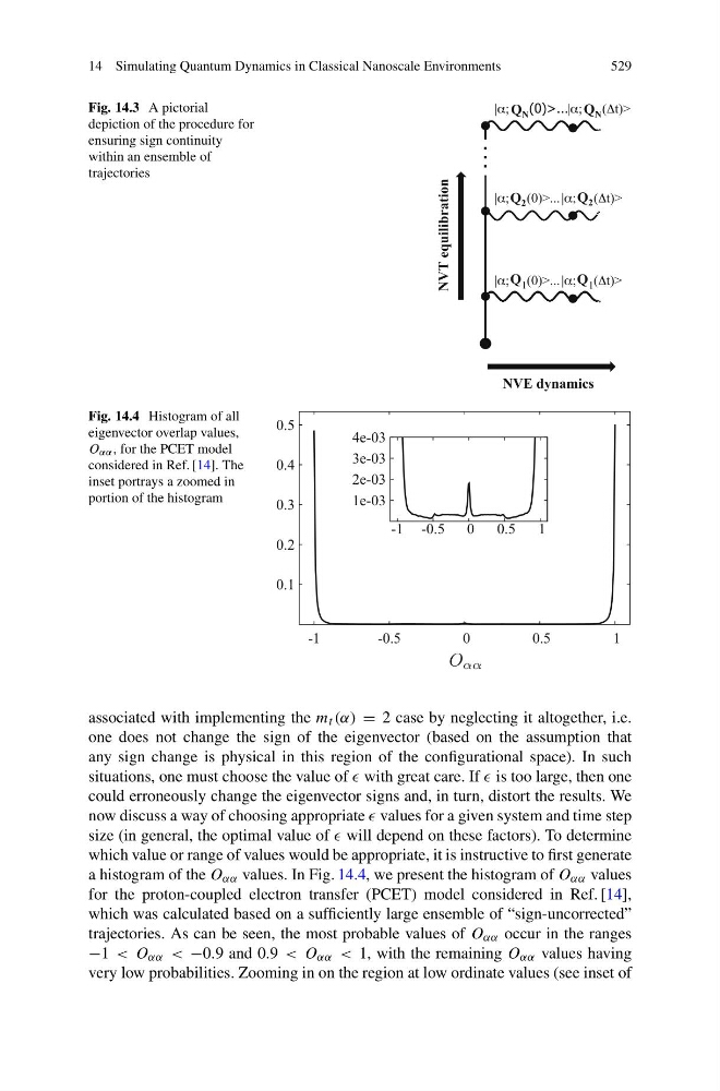
Fig. 14.4 Histogram of all
eigenvector overlap values,
O αα , for the PCET model
considered in Ref. [14]. The
inset portrays a zoomed in
portion of the histogram
0.1
0.2
0.3
0.4
0.5
-1
-0.5
0
0.5
1
1e-03
2e-03
3e-03
4e-03
-1 -0.5 0
0.5
1
O αα
associated with implementing the m t (α) = 2 case by neglecting it altogether, i.e.
one does not change the sign of the eigenvector (based on the assumption that
any sign change is physical in this region of the configurational space). In such
situations, one must choose the value of with great care. If is too large, then one
could erroneously change the eigenvector signs and, in turn, distort the results. We
now discuss a way of choosing appropriate values for a given system and time step
size (in general, the optimal value of will depend on these factors). To determine
which value or range of values would be appropriate, it is instructive to first generate
a histogram of the O αα values. In Fig. 14.4, we present the histogram of O αα values
for the proton-coupled electron transfer (PCET) model considered in Ref. [14],
which was calculated based on a sufficiently large ensemble of “sign-uncorrected”
trajectories. As can be seen, the most probable values of O αα occur in the ranges
−1 < O αα < −0.9 and 0.9 < O αα < 1, with the remaining O αα values having
very low probabilities. Zooming in on the region at low ordinate values (see inset of
529
Fig. 14.3 A pictorial
depiction of the procedure for
ensuring sign continuity
within an ensemble of
trajectories
Fig. 14.4 Histogram of all
eigenvector overlap values,
O αα , for the PCET model
considered in Ref. [14]. The
inset portrays a zoomed in
portion of the histogram
0.1
0.2
0.3
0.4
0.5
-1
-0.5
0
0.5
1
1e-03
2e-03
3e-03
4e-03
-1 -0.5 0
0.5
1
O αα
associated with implementing the m t (α) = 2 case by neglecting it altogether, i.e.
one does not change the sign of the eigenvector (based on the assumption that
any sign change is physical in this region of the configurational space). In such
situations, one must choose the value of with great care. If is too large, then one
could erroneously change the eigenvector signs and, in turn, distort the results. We
now discuss a way of choosing appropriate values for a given system and time step
size (in general, the optimal value of will depend on these factors). To determine
which value or range of values would be appropriate, it is instructive to first generate
a histogram of the O αα values. In Fig. 14.4, we present the histogram of O αα values
for the proton-coupled electron transfer (PCET) model considered in Ref. [14],
which was calculated based on a sufficiently large ensemble of “sign-uncorrected”
trajectories. As can be seen, the most probable values of O αα occur in the ranges
−1 < O αα < −0.9 and 0.9 < O αα < 1, with the remaining O αα values having
very low probabilities. Zooming in on the region at low ordinate values (see inset of