

526
G. Hanna and A. Sergi
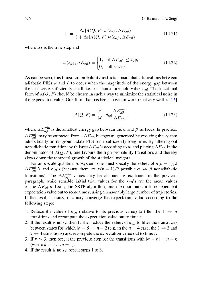
=
t|A(Q, P )|w(κ αβ , ,E αβ )
1 + t|A(Q, P )|w(κ αβ , ,E αβ )
,
(14.21)
where t is the time step and
w(κ αβ , ,E αβ ) =
1, if|E αβ | ≤ κ αβ ,
0, otherwise.
(14.22)
As can be seen, this transition probability restricts nonadiabatic transitions between
adiabatic PESs α and β to occur when the magnitude of the energy gap between
the surfaces is sufficiently small, i.e. less than a threshold value κ αβ . The functional
form of A(Q, P ) should be chosen in such a way to minimize the statistical noise in
the expectation value. One form that has been shown to work relatively well is [12]
A(Q, P ) =
P
M
· d αβ
E min
αβ
E αβ
,
(14.23)
where E min
αβ is the smallest energy gap between the α and β surfaces. In practice,
E min
αβ may be extracted from a E αβ histogram, generated by evolving the system
adiabatically on its ground-state PES for a sufficiently long time. By filtering out
nonadiabatic transitions with large E αβ ’s according to w and placing E αβ in the
denominator of A(Q, P ), one favours the high-probability transitions and thereby
slows down the temporal growth of the statistical weights.
For an n-state quantum subsystem, one must specify the values of n(n − 1)/2
E min
αβ ’s and κ αβ ’s (because there are n(n − 1)/2 possible α ↔ β nonadiabatic
transitions). The E min
αβ values may be obtained as explained in the previous
paragraph, while sensible initial trial values for the κ αβ ’s are the mean values
of the E αβ ’s. Using the SSTP algorithm, one then computes a time-dependent
expectation value out to some time t, using a reasonably large number of trajectories.
If the result is noisy, one may converge the expectation value according to the
following steps:
1. Reduce the value of κ 1n (relative to its previous value) to filter the 1 ↔ n
transitions and recompute the expectation value out to time t.
2. If the result is noisy, then further reduce the values of κ αβ to filter the transitions
between states for which |α − β| = n − 2 (e.g. in the n = 4 case, the 1 ↔ 3 and
2 ↔ 4 transitions) and recompute the expectation value out to time t.
3. If n > 3, then repeat the previous step for the transitions with |α − β| = n − k
(where k = 3 . . . n − 1).
4. If the result is noisy, repeat steps 1 to 3.
G. Hanna and A. Sergi
=
t|A(Q, P )|w(κ αβ , ,E αβ )
1 + t|A(Q, P )|w(κ αβ , ,E αβ )
,
(14.21)
where t is the time step and
w(κ αβ , ,E αβ ) =
1, if|E αβ | ≤ κ αβ ,
0, otherwise.
(14.22)
As can be seen, this transition probability restricts nonadiabatic transitions between
adiabatic PESs α and β to occur when the magnitude of the energy gap between
the surfaces is sufficiently small, i.e. less than a threshold value κ αβ . The functional
form of A(Q, P ) should be chosen in such a way to minimize the statistical noise in
the expectation value. One form that has been shown to work relatively well is [12]
A(Q, P ) =
P
M
· d αβ
E min
αβ
E αβ
,
(14.23)
where E min
αβ is the smallest energy gap between the α and β surfaces. In practice,
E min
αβ may be extracted from a E αβ histogram, generated by evolving the system
adiabatically on its ground-state PES for a sufficiently long time. By filtering out
nonadiabatic transitions with large E αβ ’s according to w and placing E αβ in the
denominator of A(Q, P ), one favours the high-probability transitions and thereby
slows down the temporal growth of the statistical weights.
For an n-state quantum subsystem, one must specify the values of n(n − 1)/2
E min
αβ ’s and κ αβ ’s (because there are n(n − 1)/2 possible α ↔ β nonadiabatic
transitions). The E min
αβ values may be obtained as explained in the previous
paragraph, while sensible initial trial values for the κ αβ ’s are the mean values
of the E αβ ’s. Using the SSTP algorithm, one then computes a time-dependent
expectation value out to some time t, using a reasonably large number of trajectories.
If the result is noisy, one may converge the expectation value according to the
following steps:
1. Reduce the value of κ 1n (relative to its previous value) to filter the 1 ↔ n
transitions and recompute the expectation value out to time t.
2. If the result is noisy, then further reduce the values of κ αβ to filter the transitions
between states for which |α − β| = n − 2 (e.g. in the n = 4 case, the 1 ↔ 3 and
2 ↔ 4 transitions) and recompute the expectation value out to time t.
3. If n > 3, then repeat the previous step for the transitions with |α − β| = n − k
(where k = 3 . . . n − 1).
4. If the result is noisy, repeat steps 1 to 3.