

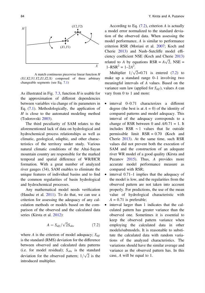
As illustrated in Fig. 7.3, function H is usable for
the approximation of different dependencies
between variables via change of its parameters in
Eq. (7.1). Methodologically, the application of
H is close to the automated modeling method
(Todorovski 2003).
The third peculiarity of SAM relates to the
aforementioned lack of data on hydrological and
hydrochemical process relationships as well as
climatic, geological, edaphic, and other characteristics of the territory under study. Various
natural climatic conditions of the Altai-Sayan
mountain country are responsible for the marked
temporal and spatial difference of WR/HCR
formation. With a great number of analyzed
river gauges (34), SAM enables to eliminate the
unique features of individual basins and to find
the common regularities of basin hydrological
and hydrochemical processes.
Any mathematical model needs verification
(Hauduc et al. 2011). To do that, we can use a
criterion for assessing the adequacy of any calculation methods or models based on the comparison of the observed and the calculated data
series (Kirsta et al. 2012):
A ¼ S dif =
ffiffi ffi
2
p
S obs
ð7:2Þ
where A is the criterion of model adequacy; S dif
is the standard (RMS) deviation for the difference
between observed and calculated data patterns
(i.e. for model residual); S obs is the standard
deviation for the observed pattern; 1=
ffiffi ffi
2
p
is the
introduced multiplier.
According to Eq. (7.2), criterion A is actually
a model error normalized to the standard deviation of the observed data. When assessing the
model performance, A is similar to performance
criterion RSR (Moriasi et al. 2007; Koch and
Cherie 2013) and Nash–Sutcliffe model efficiency coefficient NSE (Koch and Cherie 2013)
related to A by equations RSR = A
ffiffi ffi
2
p
, NSE =
1–RSR
2 = 1–2A
2 .
Multiplier 1=
ffiffi ffi
2
p
=0.71 is entered (7.2) to
make up a standard range 0–1 involving two
meaningful intervals of A values. Based on the
variance sum law (applied for S dif ), values A can
vary from 0 to 1 and more:
• interval 0–0.71 characterizes a different
degree (the best is at A = 0) of the identity of
compared patterns and model adequacy. This
interval of the adequacy corresponds to a
change of RSR between 0 and A/0.71 = 1. It
includes RSR *1 values that lie outside
permissible limit RSR = 0.70 (Koch and
Cherie 2013). At the same time, such RSR
values did not prevent both the execution of
SAM and the construction of an adequate
river WR model of a good quality (Kirsta and
Puzanov 2015). Thus, A provides more
accurate model performance measure as
compared with RSR;
• interval 0.71–1 implies that the adequacy of
the model is low, and the regularities from the
observed pattern are not taken into account
properly. For predictions, the use of the mean
value of hydrological characteristic with
A = 0.71 is preferable;
• interval larger than 1 indicates that the calculated pattern has greater variance than the
observed one. Sometimes it is essential to
keep the observed pattern variance when
employing the calculated data in other
models/submodels. It is reasonable to substitute the calculated data with random variations of the analyzed characteristics. The
variations should have the similar average and
variance as the observed pattern has. In this
case, A will be equal to 1.
X
H
(X1,Y1)
(X 2,Y2)
Fig. 7.3 A match continuous piecewise linear function H
(X1,X2,Y1,Y2,Z1,Z2,X) composed of three arbitrary
changeable segments (see Eq. 7.1)
84
Y. Kirsta and A. Puzanov
the approximation of different dependencies
between variables via change of its parameters in
Eq. (7.1). Methodologically, the application of
H is close to the automated modeling method
(Todorovski 2003).
The third peculiarity of SAM relates to the
aforementioned lack of data on hydrological and
hydrochemical process relationships as well as
climatic, geological, edaphic, and other characteristics of the territory under study. Various
natural climatic conditions of the Altai-Sayan
mountain country are responsible for the marked
temporal and spatial difference of WR/HCR
formation. With a great number of analyzed
river gauges (34), SAM enables to eliminate the
unique features of individual basins and to find
the common regularities of basin hydrological
and hydrochemical processes.
Any mathematical model needs verification
(Hauduc et al. 2011). To do that, we can use a
criterion for assessing the adequacy of any calculation methods or models based on the comparison of the observed and the calculated data
series (Kirsta et al. 2012):
A ¼ S dif =
ffiffi ffi
2
p
S obs
ð7:2Þ
where A is the criterion of model adequacy; S dif
is the standard (RMS) deviation for the difference
between observed and calculated data patterns
(i.e. for model residual); S obs is the standard
deviation for the observed pattern; 1=
ffiffi ffi
2
p
is the
introduced multiplier.
According to Eq. (7.2), criterion A is actually
a model error normalized to the standard deviation of the observed data. When assessing the
model performance, A is similar to performance
criterion RSR (Moriasi et al. 2007; Koch and
Cherie 2013) and Nash–Sutcliffe model efficiency coefficient NSE (Koch and Cherie 2013)
related to A by equations RSR = A
ffiffi ffi
2
p
, NSE =
1–RSR
2 = 1–2A
2 .
Multiplier 1=
ffiffi ffi
2
p
=0.71 is entered (7.2) to
make up a standard range 0–1 involving two
meaningful intervals of A values. Based on the
variance sum law (applied for S dif ), values A can
vary from 0 to 1 and more:
• interval 0–0.71 characterizes a different
degree (the best is at A = 0) of the identity of
compared patterns and model adequacy. This
interval of the adequacy corresponds to a
change of RSR between 0 and A/0.71 = 1. It
includes RSR *1 values that lie outside
permissible limit RSR = 0.70 (Koch and
Cherie 2013). At the same time, such RSR
values did not prevent both the execution of
SAM and the construction of an adequate
river WR model of a good quality (Kirsta and
Puzanov 2015). Thus, A provides more
accurate model performance measure as
compared with RSR;
• interval 0.71–1 implies that the adequacy of
the model is low, and the regularities from the
observed pattern are not taken into account
properly. For predictions, the use of the mean
value of hydrological characteristic with
A = 0.71 is preferable;
• interval larger than 1 indicates that the calculated pattern has greater variance than the
observed one. Sometimes it is essential to
keep the observed pattern variance when
employing the calculated data in other
models/submodels. It is reasonable to substitute the calculated data with random variations of the analyzed characteristics. The
variations should have the similar average and
variance as the observed pattern has. In this
case, A will be equal to 1.
X
H
(X1,Y1)
(X 2,Y2)
Fig. 7.3 A match continuous piecewise linear function H
(X1,X2,Y1,Y2,Z1,Z2,X) composed of three arbitrary
changeable segments (see Eq. 7.1)
84
Y. Kirsta and A. Puzanov