

steppe high, middle and low mountains to the
streamflow during summer and autumn low
water (geosystem groups 4, 6 in seasons 3, 4).
By and large values of b k show that over half of
precipitation enters the river streamflow in summer low water and slightly less than half—during
autumn low water period.
In turn, values of c 10 in Eq. (7.3) characterizing the continuous replenishment or leakage of
streamflow into groundwater and/or into water of
rock fracture zones are + 0.27; + 0.40; –0.02; –
0.38 for 1–4 seasons, correspondingly, i.e.
+ 27%, + 40%, –2%, –38% of the long-term
mean river basin runoff. Here one can see small
water outflow into groundwater during summer
(–2%); i.e. summer feeding of rivers in the AltaiSayan mountain country is provided mainly by
precipitation of previous and current hydrological seasons.
Using the calculated and observed streamflow
patterns, we can estimate the adequacy of the
developed simulation balance WR model (7.3)
by criterion A in (7.2). A values calculated for
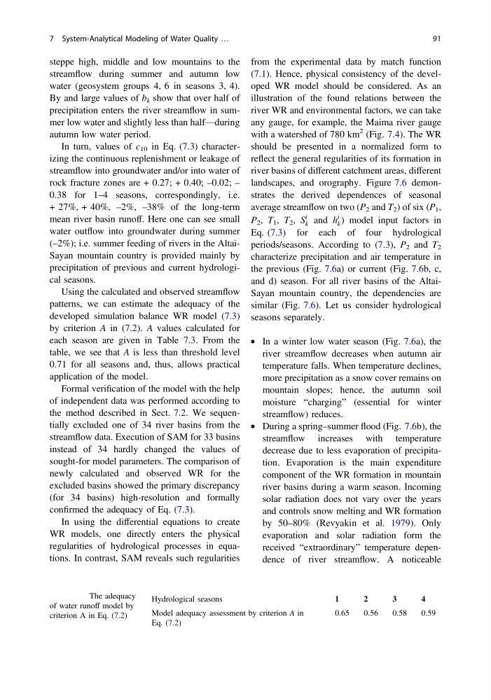
each season are given in Table 7.3. From the
table, we see that A is less than threshold level
0.71 for all seasons and, thus, allows practical
application of the model.
Formal verification of the model with the help
of independent data was performed according to
the method described in Sect. 7.2. We sequentially excluded one of 34 river basins from the
streamflow data. Execution of SAM for 33 basins
instead of 34 hardly changed the values of
sought-for model parameters. The comparison of
newly calculated and observed WR for the
excluded basins showed the primary discrepancy
(for 34 basins) high-resolution and formally
confirmed the adequacy of Eq. (7.3).
In using the differential equations to create
WR models, one directly enters the physical
regularities of hydrological processes in equations. In contrast, SAM reveals such regularities
from the experimental data by match function
(7.1). Hence, physical consistency of the developed WR model should be considered. As an
illustration of the found relations between the
river WR and environmental factors, we can take
any gauge, for example, the Maima river gauge
with a watershed of 780 km
2 (Fig. 7.4). The WR
should be presented in a normalized form to
reflect the general regularities of its formation in
river basins of different catchment areas, different
landscapes, and orography. Figure 7.6 demonstrates the derived dependences of seasonal
average streamflow on two (P 2 and T 2 ) of six (P 1 ,
P 2 , T 1 , T 2 , S
i
k and h
i
k ) model input factors in
Eq. (7.3) for each of four hydrological
periods/seasons. According to (7.3), P 2 and T 2
characterize precipitation and air temperature in
the previous (Fig. 7.6a) or current (Fig. 7.6b, c,
and d) season. For all river basins of the AltaiSayan mountain country, the dependencies are
similar (Fig. 7.6). Let us consider hydrological
seasons separately.
• In a winter low water season (Fig. 7.6a), the
river streamflow decreases when autumn air
temperature falls. When temperature declines,
more precipitation as a snow cover remains on
mountain slopes; hence, the autumn soil
moisture “charging” (essential for winter
streamflow) reduces.
• During a spring–summer flood (Fig. 7.6b), the
streamflow increases with temperature
decrease due to less evaporation of precipitation. Evaporation is the main expenditure
component of the WR formation in mountain
river basins during a warm season. Incoming
solar radiation does not vary over the years
and controls snow melting and WR formation
by 50–80% (Revyakin et al. 1979). Only
evaporation and solar radiation form the
received “extraordinary” temperature dependence of river streamflow. A noticeable
Table 7.3 The adequacy
of water runoff model by
criterion A in Eq. (7.2)
Hydrological seasons
1
2
3
4
Model adequacy assessment by criterion A in
Eq. (7.2)
0.65
0.56
0.58
0.59
7 System-Analytical Modeling of Water Quality …
91
streamflow during summer and autumn low
water (geosystem groups 4, 6 in seasons 3, 4).
By and large values of b k show that over half of
precipitation enters the river streamflow in summer low water and slightly less than half—during
autumn low water period.
In turn, values of c 10 in Eq. (7.3) characterizing the continuous replenishment or leakage of
streamflow into groundwater and/or into water of
rock fracture zones are + 0.27; + 0.40; –0.02; –
0.38 for 1–4 seasons, correspondingly, i.e.
+ 27%, + 40%, –2%, –38% of the long-term
mean river basin runoff. Here one can see small
water outflow into groundwater during summer
(–2%); i.e. summer feeding of rivers in the AltaiSayan mountain country is provided mainly by
precipitation of previous and current hydrological seasons.
Using the calculated and observed streamflow
patterns, we can estimate the adequacy of the
developed simulation balance WR model (7.3)
by criterion A in (7.2). A values calculated for
each season are given in Table 7.3. From the
table, we see that A is less than threshold level
0.71 for all seasons and, thus, allows practical
application of the model.
Formal verification of the model with the help
of independent data was performed according to
the method described in Sect. 7.2. We sequentially excluded one of 34 river basins from the
streamflow data. Execution of SAM for 33 basins
instead of 34 hardly changed the values of
sought-for model parameters. The comparison of
newly calculated and observed WR for the
excluded basins showed the primary discrepancy
(for 34 basins) high-resolution and formally
confirmed the adequacy of Eq. (7.3).
In using the differential equations to create
WR models, one directly enters the physical
regularities of hydrological processes in equations. In contrast, SAM reveals such regularities
from the experimental data by match function
(7.1). Hence, physical consistency of the developed WR model should be considered. As an
illustration of the found relations between the
river WR and environmental factors, we can take
any gauge, for example, the Maima river gauge
with a watershed of 780 km
2 (Fig. 7.4). The WR
should be presented in a normalized form to
reflect the general regularities of its formation in
river basins of different catchment areas, different
landscapes, and orography. Figure 7.6 demonstrates the derived dependences of seasonal
average streamflow on two (P 2 and T 2 ) of six (P 1 ,
P 2 , T 1 , T 2 , S
i
k and h
i
k ) model input factors in
Eq. (7.3) for each of four hydrological
periods/seasons. According to (7.3), P 2 and T 2
characterize precipitation and air temperature in
the previous (Fig. 7.6a) or current (Fig. 7.6b, c,
and d) season. For all river basins of the AltaiSayan mountain country, the dependencies are
similar (Fig. 7.6). Let us consider hydrological
seasons separately.
• In a winter low water season (Fig. 7.6a), the
river streamflow decreases when autumn air
temperature falls. When temperature declines,
more precipitation as a snow cover remains on
mountain slopes; hence, the autumn soil
moisture “charging” (essential for winter
streamflow) reduces.
• During a spring–summer flood (Fig. 7.6b), the
streamflow increases with temperature
decrease due to less evaporation of precipitation. Evaporation is the main expenditure
component of the WR formation in mountain
river basins during a warm season. Incoming
solar radiation does not vary over the years
and controls snow melting and WR formation
by 50–80% (Revyakin et al. 1979). Only
evaporation and solar radiation form the
received “extraordinary” temperature dependence of river streamflow. A noticeable
Table 7.3 The adequacy
of water runoff model by
criterion A in Eq. (7.2)
Hydrological seasons
1
2
3
4
Model adequacy assessment by criterion A in
Eq. (7.2)
0.65
0.56
0.58
0.59
7 System-Analytical Modeling of Water Quality …
91