

407
change. Figure 20.2 shows the primary data variability as well as information that
revealed the concerns in dynamic land degradation, variety, and land use. In the examination, secondary information and information from, for instance, literature review,
different government statistics, and population censuses could complement the above.
In addition, the information is slightly different from every other source. Several spatial
sampling methods were urged by the spatial distribution data to be useful, particularly
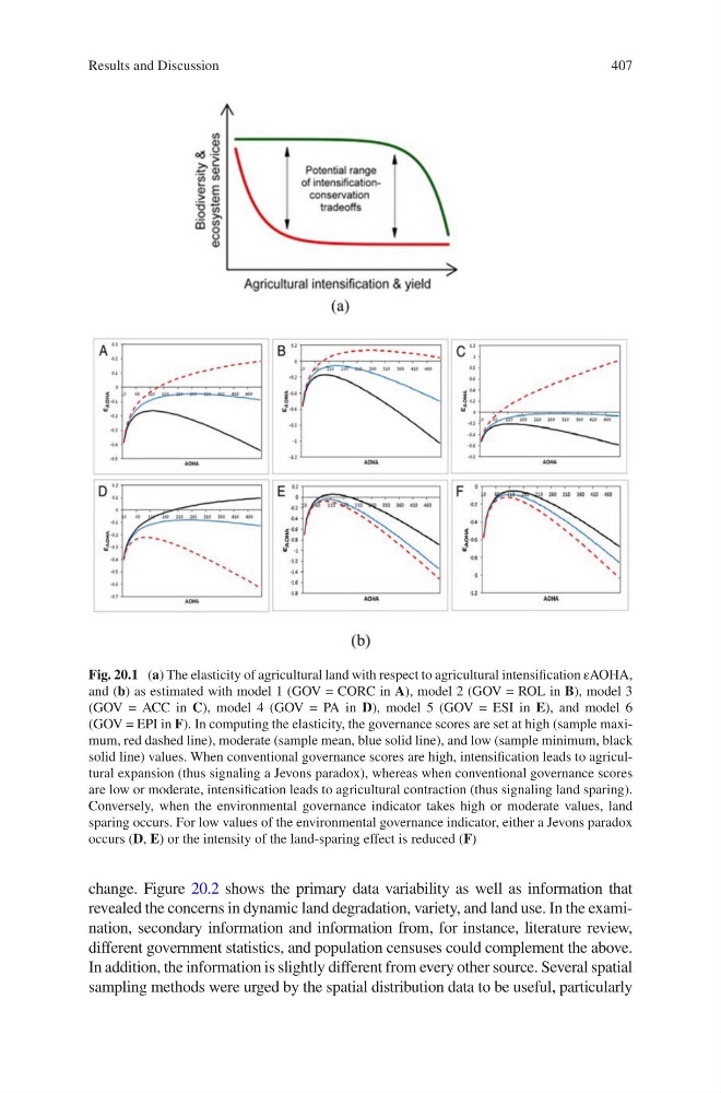
Fig. 20.1 (a) The elasticity of agricultural land with respect to agricultural intensification εAOHA,
and (b) as estimated with model 1 (GOV = CORC in A), model 2 (GOV = ROL in B), model 3
(GOV = ACC in C), model 4 (GOV = PA in D), model 5 (GOV = ESI in E), and model 6
(GOV = EPI in F). In computing the elasticity, the governance scores are set at high (sample maximum, red dashed line), moderate (sample mean, blue solid line), and low (sample minimum, black
solid line) values. When conventional governance scores are high, intensification leads to agricultural expansion (thus signaling a Jevons paradox), whereas when conventional governance scores
are low or moderate, intensification leads to agricultural contraction (thus signaling land sparing).
Conversely, when the environmental governance indicator takes high or moderate values, land
sparing occurs. For low values of the environmental governance indicator, either a Jevons paradox
occurs (D, E) or the intensity of the land-sparing effect is reduced (F)
Results and Discussion
change. Figure 20.2 shows the primary data variability as well as information that
revealed the concerns in dynamic land degradation, variety, and land use. In the examination, secondary information and information from, for instance, literature review,
different government statistics, and population censuses could complement the above.
In addition, the information is slightly different from every other source. Several spatial
sampling methods were urged by the spatial distribution data to be useful, particularly
Fig. 20.1 (a) The elasticity of agricultural land with respect to agricultural intensification εAOHA,
and (b) as estimated with model 1 (GOV = CORC in A), model 2 (GOV = ROL in B), model 3
(GOV = ACC in C), model 4 (GOV = PA in D), model 5 (GOV = ESI in E), and model 6
(GOV = EPI in F). In computing the elasticity, the governance scores are set at high (sample maximum, red dashed line), moderate (sample mean, blue solid line), and low (sample minimum, black
solid line) values. When conventional governance scores are high, intensification leads to agricultural expansion (thus signaling a Jevons paradox), whereas when conventional governance scores
are low or moderate, intensification leads to agricultural contraction (thus signaling land sparing).
Conversely, when the environmental governance indicator takes high or moderate values, land
sparing occurs. For low values of the environmental governance indicator, either a Jevons paradox
occurs (D, E) or the intensity of the land-sparing effect is reduced (F)
Results and Discussion