

203
Solving the Concept Numerically
As discussed earlier, the 3D standard k-omega turbulence model is based on the
transport velocity model as an empirical model in assuring accurate dissipation
rates and for turbulence kinetic energy and is indicated in Eq. (11.2):
ψ
θ
= −
+
−
∞
∞
∞
v r r
r
v r r
v r
o
o
o
2
2
2
4
3
4
2
sin
(11.1)
v v
r
r
r
r
r
o
o
=
−
+
∞ 1
3
2
1
2
3
cosθ
(11.2)
v
v
r
r
r
r
θ
θ
= −
−
−
∞ 1
3
4
1
4
3
o
o
sin
(11.3)
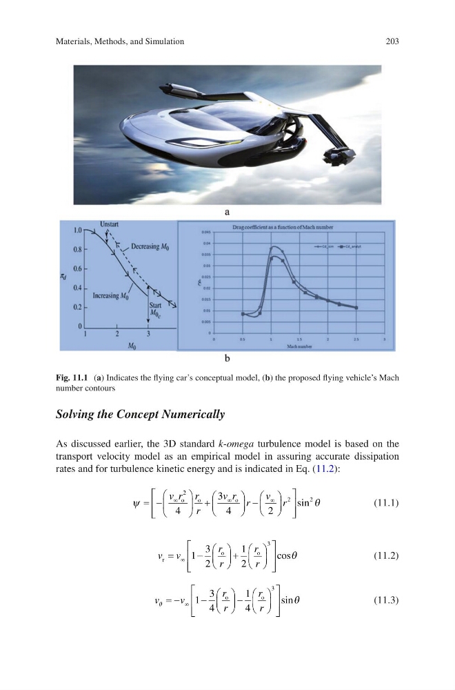
Fig. 11.1 (a) Indicates the flying car’s conceptual model, (b) the proposed flying vehicle’s Mach
number contours
Materials, Methods, and Simulation
Solving the Concept Numerically
As discussed earlier, the 3D standard k-omega turbulence model is based on the
transport velocity model as an empirical model in assuring accurate dissipation
rates and for turbulence kinetic energy and is indicated in Eq. (11.2):
ψ
θ
= −
+
−
∞
∞
∞
v r r
r
v r r
v r
o
o
o
2
2
2
4
3
4
2
sin
(11.1)
v v
r
r
r
r
r
o
o
=
−
+
∞ 1
3
2
1
2
3
cosθ
(11.2)
v
v
r
r
r
r
θ
θ
= −
−
−
∞ 1
3
4
1
4
3
o
o
sin
(11.3)
Fig. 11.1 (a) Indicates the flying car’s conceptual model, (b) the proposed flying vehicle’s Mach
number contours
Materials, Methods, and Simulation