

97
φ S
S
S
S
0
0
3
2
0
5
2
0
2
3
1
5
3
1
1507
420
1
[ ]=
−
(
) +
−
(
)
−
(
–
) ) +…(
)
7
2
0
1 1
S –
.
(5.39)
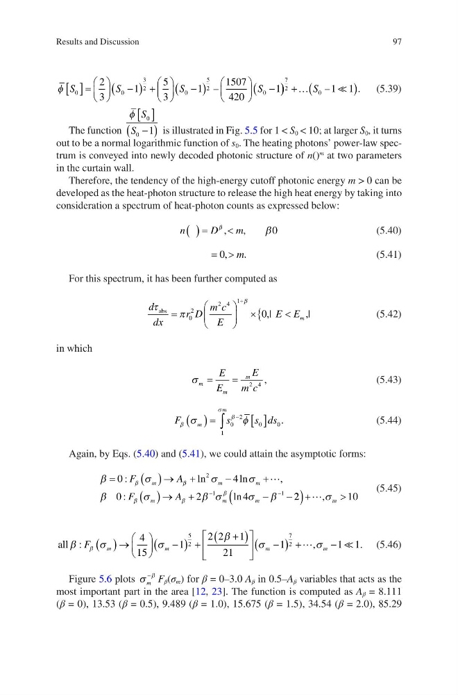
The function
φ S
S
0
0
1
[ ]
−
(
) is illustrated in Fig. 5.5 for 1 < S 0 < 10; at larger S 0 , it turns
out to be a normal logarithmic function of s 0 . The heating photons’ power-law spectrum is conveyed into newly decoded photonic structure of n()
m
at two parameters
in the curtain wall.
Therefore, the tendency of the high-energy cutoff photonic energy m > 0 can be
developed as the heat-photon structure to release the high heat energy by taking into
consideration a spectrum of heat-photon counts as expressed below:
n
D
m
( ) = <
β
β
,
,
0
(5.40)
= >
0,
.
m
(5.41)
For this spectrum, it has been further computed as
d
dx
r D
m c
E
E E m
τ
π
β
abs
,|
,|
=
×
<
{
+
0
2
2 4 1
0
(5.42)
in which
σ m
m
m
E
E
E
m c
=
= 2 4 ,
(5.43)
F
s
s ds
m
m
β
σ
β
σ
φ
( )=
[ ]
∫
−
1
0
2
0
0 .
(5.44)
Again, by Eqs. (5.40) and (5.41), we could attain the asymptotic forms:
β
σ
σ
σ
β
σ
β σ
σ
β
β
β
β
β
β
=
( )→ +
−
+
( )→ +
−
−
−
−
0
4
0
2
4
2
1
1
:
l n
l n
,
:
l n
F
A
F
A
m
m
m
m
m
m
2 2
1 0
(
) +
>
,σ m
(5.45)
all β
σ
σ
β
σ
σ
β
:
,
F
m
m
m
m
( )→
−
(
) +
+
(
)
−
(
) +
4
15
1
2 2
1
21
1
5
2
7
2
− −1 1
. (5.46)
Figure 5.6 plots σ
β
m
− F β (σ m ) for β = 0–3.0 A β in 0.5–A β variables that acts as the
most important part in the area [12, 23]. The function is computed as A β = 8.111
(β = 0), 13.53 (β = 0.5), 9.489 (β = 1.0), 15.675 (β = 1.5), 34.54 (β = 2.0), 85.29
Results and Discussion
φ S
S
S
S
0
0
3
2
0
5
2
0
2
3
1
5
3
1
1507
420
1
[ ]=
−
(
) +
−
(
)
−
(
–
) ) +…(
)
7
2
0
1 1
S –
.
(5.39)
The function
φ S
S
0
0
1
[ ]
−
(
) is illustrated in Fig. 5.5 for 1 < S 0 < 10; at larger S 0 , it turns
out to be a normal logarithmic function of s 0 . The heating photons’ power-law spectrum is conveyed into newly decoded photonic structure of n()
m
at two parameters
in the curtain wall.
Therefore, the tendency of the high-energy cutoff photonic energy m > 0 can be
developed as the heat-photon structure to release the high heat energy by taking into
consideration a spectrum of heat-photon counts as expressed below:
n
D
m
( ) = <
β
β
,
,
0
(5.40)
= >
0,
.
m
(5.41)
For this spectrum, it has been further computed as
d
dx
r D
m c
E
E E m
τ
π
β
abs
,|
,|
=
×
<
{
+
0
2
2 4 1
0
(5.42)
in which
σ m
m
m
E
E
E
m c
=
= 2 4 ,
(5.43)
F
s
s ds
m
m
β
σ
β
σ
φ
( )=
[ ]
∫
−
1
0
2
0
0 .
(5.44)
Again, by Eqs. (5.40) and (5.41), we could attain the asymptotic forms:
β
σ
σ
σ
β
σ
β σ
σ
β
β
β
β
β
β
=
( )→ +
−
+
( )→ +
−
−
−
−
0
4
0
2
4
2
1
1
:
l n
l n
,
:
l n
F
A
F
A
m
m
m
m
m
m
2 2
1 0
(
) +
>
,σ m
(5.45)
all β
σ
σ
β
σ
σ
β
:
,
F
m
m
m
m
( )→
−
(
) +
+
(
)
−
(
) +
4
15
1
2 2
1
21
1
5
2
7
2
− −1 1
. (5.46)
Figure 5.6 plots σ
β
m
− F β (σ m ) for β = 0–3.0 A β in 0.5–A β variables that acts as the
most important part in the area [12, 23]. The function is computed as A β = 8.111
(β = 0), 13.53 (β = 0.5), 9.489 (β = 1.0), 15.675 (β = 1.5), 34.54 (β = 2.0), 85.29
Results and Discussion