

1.9 Electrocapillary Curves of Liquid and Solid Metal Electrodes
25
0.45
0.40
0.35
0.30
0.25
/ J m
-2
-1.0 -0.5 0.0
0.5
1.0
(E - E pzc ) / V
ecm
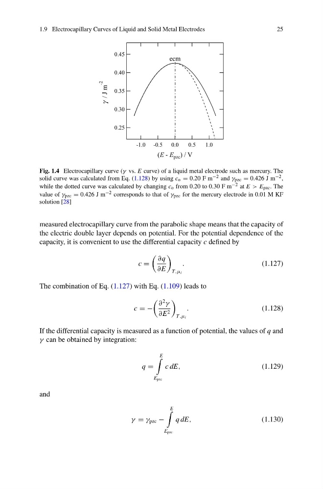
Fig. 1.4 Electrocapillary curve (γ vs. E curve) of a liquid metal electrode such as mercury. The
solid curve was calculated from Eq. (1.128) by using c o = 0.20 F m −2 and γ pzc = 0.426 J m −2 ,
while the dotted curve was calculated by changing c o from 0.20 to 0.30 F m −2 at E > E pzc . The
value of γ pzc = 0.426 J m −2 corresponds to that of γ pzc for the mercury electrode in 0.01 M KF
solution [28]
measured electrocapillary curve from the parabolic shape means that the capacity of
the electric double layer depends on potential. For the potential dependence of the
capacity, it is convenient to use the differential capacity c defined by
c =
∂q
∂E
T ,μ i
.
(1.127)
The combination of Eq. (1.127) with Eq. (1.109) leads to
c = −
∂
2
γ
∂E 2
T ,μ i
.
(1.128)
If the differential capacity is measured as a function of potential, the values of q and
γ can be obtained by integration:
q =
E
E pzc
c dE,
(1.129)
and
γ = γ pzc −
E
E pzc
q dE,
(1.130)
25
0.45
0.40
0.35
0.30
0.25
/ J m
-2
-1.0 -0.5 0.0
0.5
1.0
(E - E pzc ) / V
ecm
Fig. 1.4 Electrocapillary curve (γ vs. E curve) of a liquid metal electrode such as mercury. The
solid curve was calculated from Eq. (1.128) by using c o = 0.20 F m −2 and γ pzc = 0.426 J m −2 ,
while the dotted curve was calculated by changing c o from 0.20 to 0.30 F m −2 at E > E pzc . The
value of γ pzc = 0.426 J m −2 corresponds to that of γ pzc for the mercury electrode in 0.01 M KF
solution [28]
measured electrocapillary curve from the parabolic shape means that the capacity of
the electric double layer depends on potential. For the potential dependence of the
capacity, it is convenient to use the differential capacity c defined by
c =
∂q
∂E
T ,μ i
.
(1.127)
The combination of Eq. (1.127) with Eq. (1.109) leads to
c = −
∂
2
γ
∂E 2
T ,μ i
.
(1.128)
If the differential capacity is measured as a function of potential, the values of q and
γ can be obtained by integration:
q =
E
E pzc
c dE,
(1.129)
and
γ = γ pzc −
E
E pzc
q dE,
(1.130)