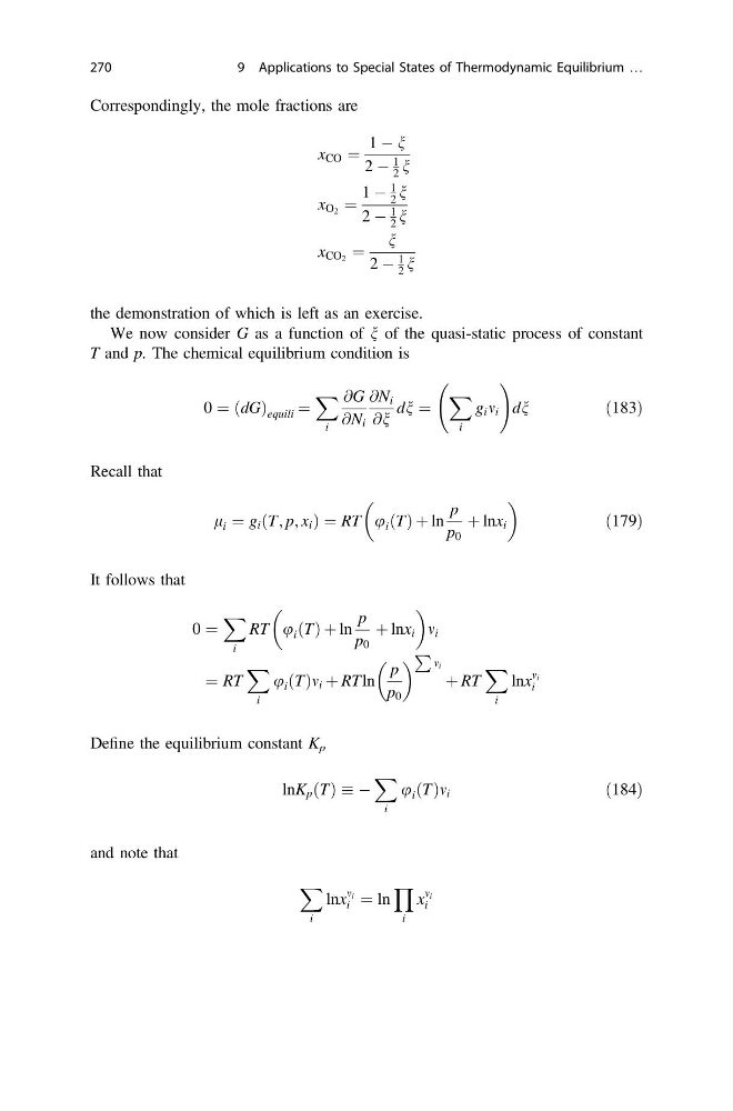
Correspondingly, the mole fractions are
x CO ¼
1 À n
2 À
1
2 n
x O 2 ¼
1 À
1
2 n
2 À
1
2 n
x CO 2 ¼
n
2 À
1
2 n
the demonstration of which is left as an exercise.
We now consider G as a function of n of the quasi-static process of constant
T and p. The chemical equilibrium condition is
0 ¼ dG
ð Þ equili ¼
X
i
@G
@N i
@N i
@n
dn ¼
X
i
g i m i
!
dn
ð183Þ
Recall that
l i ¼ g i T; p; x i
ð
Þ¼RT u i T
ð Þ þ ln
p
p 0
þ lnx i
ð179Þ
It follows that
0 ¼
X
i
RT u i T
ð Þ þ ln
p
p 0
þ lnx i
m i
¼ RT
X
i
u i T
ð Þm i þ RTln
p
p 0
P
m i
þ RT
X
i
lnx
m i
i
Define the equilibrium constant K p
lnK p T
ð Þ À
X
i
u i T
ð Þm i
ð184Þ
and note that
X
i
lnx
m i
i ¼ ln
Y
i
x
m i
i
270
9 Applications to Special States of Thermodynamic Equilibrium …