

Finally, we find
S ¼
6
2
Rln
T
1
ð Þ
250
þ S
1
ð Þ
250
ð
Þþ
15
2
Rln
450 À
2
5 T
1
ð Þ
350
þ S
2
ð Þ
350
ð
Þ
Note that U
(1)
– U
(1) (250 K) = 3R(T
(1)
– 250). A quasi-static trajectory can be
constructed in terms of [S – S
(1) (250 K) – S
(2) (350 K)] versus [U
(1)
– U
(1) (250 K)]
or U
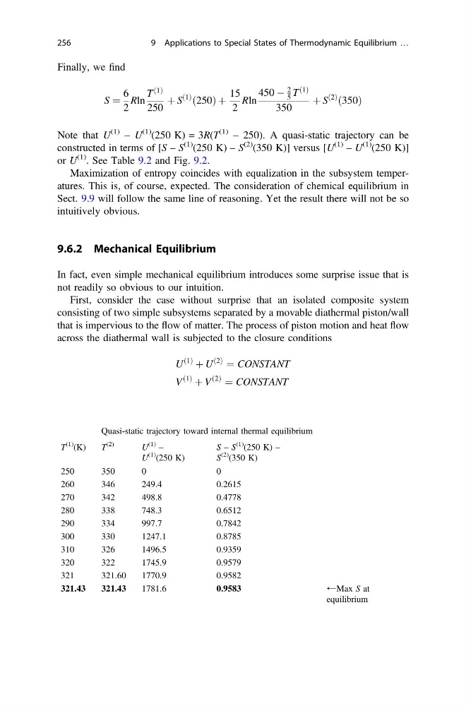
(1) . See Table 9.2 and Fig. 9.2.
Maximization of entropy coincides with equalization in the subsystem temperatures. This is, of course, expected. The consideration of chemical equilibrium in
Sect. 9.9 will follow the same line of reasoning. Yet the result there will not be so
intuitively obvious.
9.6.2 Mechanical Equilibrium
In fact, even simple mechanical equilibrium introduces some surprise issue that is
not readily so obvious to our intuition.
First, consider the case without surprise that an isolated composite system
consisting of two simple subsystems separated by a movable diathermal piston/wall
that is impervious to the flow of matter. The process of piston motion and heat flow
across the diathermal wall is subjected to the closure conditions
U
1
ð Þ
þ U
2
ð Þ
¼ CONSTANT
V
1
ð Þ
þ V
2
ð Þ
¼ CONSTANT
Table 9.2 Quasi-static trajectory toward internal thermal equilibrium
T
(1) (K)
T
(2)
U
(1) –
U
(1)
(250 K)
S – S
(1)
(250 K) –
S
(2)
(350 K)
250
350
0
0
260
346
249.4
0.2615
270
342
498.8
0.4778
280
338
748.3
0.6512
290
334
997.7
0.7842
300
330
1247.1
0.8785
310
326
1496.5
0.9359
320
322
1745.9
0.9579
321
321.60
1770.9
0.9582
321.43
321.43
1781.6
0.9583
←Max S at
equilibrium
256
9 Applications to Special States of Thermodynamic Equilibrium …
S ¼
6
2
Rln
T
1
ð Þ
250
þ S
1
ð Þ
250
ð
Þþ
15
2
Rln
450 À
2
5 T
1
ð Þ
350
þ S
2
ð Þ
350
ð
Þ
Note that U
(1)
– U
(1) (250 K) = 3R(T
(1)
– 250). A quasi-static trajectory can be
constructed in terms of [S – S
(1) (250 K) – S
(2) (350 K)] versus [U
(1)
– U
(1) (250 K)]
or U
(1) . See Table 9.2 and Fig. 9.2.
Maximization of entropy coincides with equalization in the subsystem temperatures. This is, of course, expected. The consideration of chemical equilibrium in
Sect. 9.9 will follow the same line of reasoning. Yet the result there will not be so
intuitively obvious.
9.6.2 Mechanical Equilibrium
In fact, even simple mechanical equilibrium introduces some surprise issue that is
not readily so obvious to our intuition.
First, consider the case without surprise that an isolated composite system
consisting of two simple subsystems separated by a movable diathermal piston/wall
that is impervious to the flow of matter. The process of piston motion and heat flow
across the diathermal wall is subjected to the closure conditions
U
1
ð Þ
þ U
2
ð Þ
¼ CONSTANT
V
1
ð Þ
þ V
2
ð Þ
¼ CONSTANT
Table 9.2 Quasi-static trajectory toward internal thermal equilibrium
T
(1) (K)
T
(2)
U
(1) –
U
(1)
(250 K)
S – S
(1)
(250 K) –
S
(2)
(350 K)
250
350
0
0
260
346
249.4
0.2615
270
342
498.8
0.4778
280
338
748.3
0.6512
290
334
997.7
0.7842
300
330
1247.1
0.8785
310
326
1496.5
0.9359
320
322
1745.9
0.9579
321
321.60
1770.9
0.9582
321.43
321.43
1781.6
0.9583
←Max S at
equilibrium
256
9 Applications to Special States of Thermodynamic Equilibrium …