

10
1.3.2 Cyclic Voltammetry
Cyclic voltammetry (CV) is an electrochemical technique in which the working
electrode potential changes linearly versus time until it reaches one limit and then
the potential is scanned back to the same or other limit. The current at the working
electrode is plotted versus the applied potential of the working electrode to give the
cyclic voltammogram trace. Cyclic voltammetry is highly suitable to study the
unknown system to identify processes under given conditions. The electrode potential is varied cyclically and with a constant rate between two values (in sawtoothlike fashion), and the current is recorded. Sweep rates vary between a few mV s
−1
and 10
4
V s
−1
. The resulting current-potential plot, the cyclic voltammogram, displays current peaks providing a survey over the processes occurring in the potential
range studied.
A simple redox reaction results in a characteristic voltammogram shown in
Fig. 1.7. For an ideal case involving one-electron redox couple, which remains in
equilibrium through the potential scan (called reversible reaction), the surface concentration of the oxidized and reduced species is maintained at the values required
by the Nernst equation in which the separation of peak potentials, ΔE = E pa − E pc ,
always equals to 58 mV independent of the scan rate and the anodic and cathodic
current densities are also equal. The peak current density j (in A/cm
2
) depends on
initial concentration of reduced species C red (in mol/L), diffusion coefficient of
reduced species D (in cm
2
/s), and potential rate v (in V/s) and can be calculated as
(Fig. 1.7):
j
n
D v
C
max
/
/
.
=
×
(
) ( )
2 69 10
5 3 2
1 2
red
r ed
Current density is independent of potential and increases with v
1/2
.
This type of cyclic voltammogram is formed by the interplay of diffusion and the
charge-transfer reaction; if the sweep rate is fast, double-layer charging also makes
0.15
0.10
0.05
0
–0.05
–0.10
–0.15
–2
–1
0
1
2
log (j /Am
–2 )
j = 0.1 Am
–2
b a – anodic slope
b c – cathodic slope
η
(V)
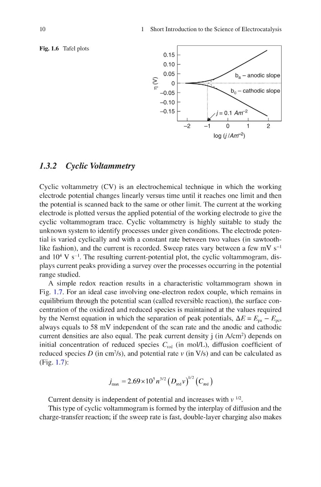
Fig. 1.6 Tafel plots
1 Short Introduction to the Science of Electrocatalysis
1.3.2 Cyclic Voltammetry
Cyclic voltammetry (CV) is an electrochemical technique in which the working
electrode potential changes linearly versus time until it reaches one limit and then
the potential is scanned back to the same or other limit. The current at the working
electrode is plotted versus the applied potential of the working electrode to give the
cyclic voltammogram trace. Cyclic voltammetry is highly suitable to study the
unknown system to identify processes under given conditions. The electrode potential is varied cyclically and with a constant rate between two values (in sawtoothlike fashion), and the current is recorded. Sweep rates vary between a few mV s
−1
and 10
4
V s
−1
. The resulting current-potential plot, the cyclic voltammogram, displays current peaks providing a survey over the processes occurring in the potential
range studied.
A simple redox reaction results in a characteristic voltammogram shown in
Fig. 1.7. For an ideal case involving one-electron redox couple, which remains in
equilibrium through the potential scan (called reversible reaction), the surface concentration of the oxidized and reduced species is maintained at the values required
by the Nernst equation in which the separation of peak potentials, ΔE = E pa − E pc ,
always equals to 58 mV independent of the scan rate and the anodic and cathodic
current densities are also equal. The peak current density j (in A/cm
2
) depends on
initial concentration of reduced species C red (in mol/L), diffusion coefficient of
reduced species D (in cm
2
/s), and potential rate v (in V/s) and can be calculated as
(Fig. 1.7):
j
n
D v
C
max
/
/
.
=
×
(
) ( )
2 69 10
5 3 2
1 2
red
r ed
Current density is independent of potential and increases with v
1/2
.
This type of cyclic voltammogram is formed by the interplay of diffusion and the
charge-transfer reaction; if the sweep rate is fast, double-layer charging also makes
0.15
0.10
0.05
0
–0.05
–0.10
–0.15
–2
–1
0
1
2
log (j /Am
–2 )
j = 0.1 Am
–2
b a – anodic slope
b c – cathodic slope
η
(V)
Fig. 1.6 Tafel plots
1 Short Introduction to the Science of Electrocatalysis