

310
6 Growth
B(0)
B G (t)
B R (t)
b(t)
B 0 (0)
F = F *
a •K•G = F *
p •G
G
F *
p
σ = 0
σ = 0
σ = 0
σ zz0
cut
e
l
b
m
e
s
s
a
e
r
w
o
r
g
load
B C (t) σ = 0
K
contract
F *
a
Passive ZSS
Active ZSS
σ p = σ p (F p
* )
σ a = σ a (F a
* )
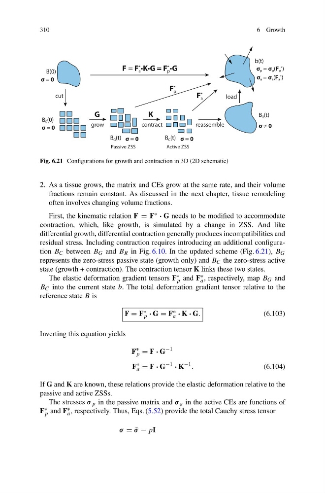
Fig. 6.21 Configurations for growth and contraction in 3D (2D schematic)
2. As a tissue grows, the matrix and CEs grow at the same rate, and their volume
fractions remain constant. As discussed in the next chapter, tissue remodeling
often involves changing volume fractions.
First, the kinematic relation F = F ∗ · G needs to be modified to accommodate
contraction, which, like growth, is simulated by a change in ZSS. And like
differential growth, differential contraction generally produces incompatibilities and
residual stress. Including contraction requires introducing an additional configuration B C between B G and B R in Fig. 6.10. In the updated scheme (Fig. 6.21), B G
represents the zero-stress passive state (growth only) and B C the zero-stress active
state (growth + contraction). The contraction tensor K links these two states.
The elastic deformation gradient tensors F ∗
p and F ∗
a , respectively, map B G and
B C into the current state b. The total deformation gradient tensor relative to the
reference state B is
F = F ∗
p · G = F ∗
a · K · G.
(6.103)
Inverting this equation yields
F
∗
p = F · G
−1
F
∗
a = F · G
−1
· K
−1 .
(6.104)
If G and K are known, these relations provide the elastic deformation relative to the
passive and active ZSSs.
The stresses σ p in the passive matrix and σ a in the active CEs are functions of
F ∗
p and F ∗
a , respectively. Thus, Eqs. (5.52) provide the total Cauchy stress tensor
σ = ¯
σ − pI
6 Growth
B(0)
B G (t)
B R (t)
b(t)
B 0 (0)
F = F *
a •K•G = F *
p •G
G
F *
p
σ = 0
σ = 0
σ = 0
σ zz0
cut
e
l
b
m
e
s
s
a
e
r
w
o
r
g
load
B C (t) σ = 0
K
contract
F *
a
Passive ZSS
Active ZSS
σ p = σ p (F p
* )
σ a = σ a (F a
* )
Fig. 6.21 Configurations for growth and contraction in 3D (2D schematic)
2. As a tissue grows, the matrix and CEs grow at the same rate, and their volume
fractions remain constant. As discussed in the next chapter, tissue remodeling
often involves changing volume fractions.
First, the kinematic relation F = F ∗ · G needs to be modified to accommodate
contraction, which, like growth, is simulated by a change in ZSS. And like
differential growth, differential contraction generally produces incompatibilities and
residual stress. Including contraction requires introducing an additional configuration B C between B G and B R in Fig. 6.10. In the updated scheme (Fig. 6.21), B G
represents the zero-stress passive state (growth only) and B C the zero-stress active
state (growth + contraction). The contraction tensor K links these two states.
The elastic deformation gradient tensors F ∗
p and F ∗
a , respectively, map B G and
B C into the current state b. The total deformation gradient tensor relative to the
reference state B is
F = F ∗
p · G = F ∗
a · K · G.
(6.103)
Inverting this equation yields
F
∗
p = F · G
−1
F
∗
a = F · G
−1
· K
−1 .
(6.104)
If G and K are known, these relations provide the elastic deformation relative to the
passive and active ZSSs.
The stresses σ p in the passive matrix and σ a in the active CEs are functions of
F ∗
p and F ∗
a , respectively. Thus, Eqs. (5.52) provide the total Cauchy stress tensor
σ = ¯
σ − pI