

246
E. Tomaszewski and M. Kozek
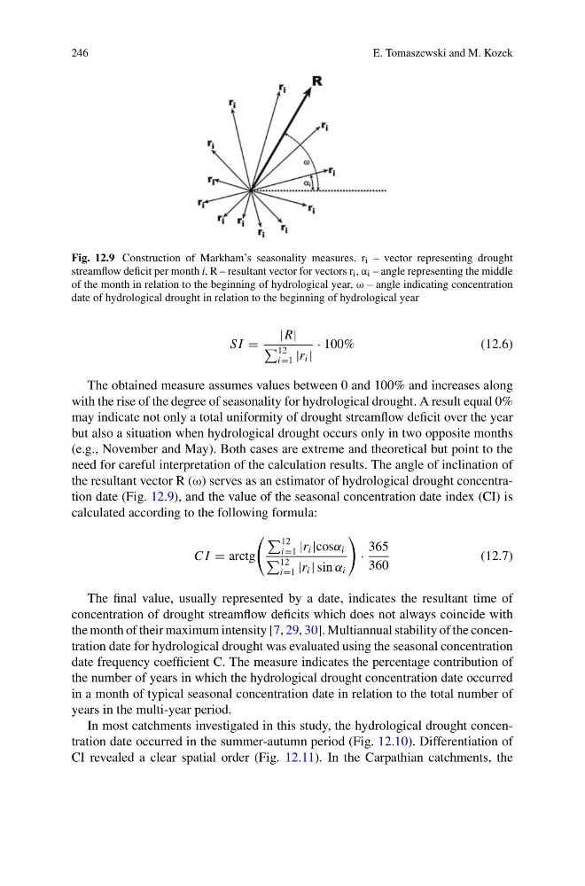
Fig. 12.9 Construction of Markham’s seasonality measures. r i – vector representing drought
streamflow deficit per month i, R – resultant vector for vectors r i , α i – angle representing the middle
of the month in relation to the beginning of hydrological year, ω – angle indicating concentration
date of hydrological drought in relation to the beginning of hydrological year
S I =
|R|
12
i=1 |r i |
· 100%
(12.6)
The obtained measure assumes values between 0 and 100% and increases along
with the rise of the degree of seasonality for hydrological drought. A result equal 0%
may indicate not only a total uniformity of drought streamflow deficit over the year
but also a situation when hydrological drought occurs only in two opposite months
(e.g., November and May). Both cases are extreme and theoretical but point to the
need for careful interpretation of the calculation results. The angle of inclination of
the resultant vector R (ω) serves as an estimator of hydrological drought concentration date (Fig. 12.9), and the value of the seasonal concentration date index (CI) is
calculated according to the following formula:
C I = arctg
12
i=1 |r i |cosα i
12
i=1 |r i | sin α i
·
365
360
(12.7)
The final value, usually represented by a date, indicates the resultant time of
concentration of drought streamflow deficits which does not always coincide with
the month of their maximum intensity [7, 29, 30]. Multiannual stability of the concentration date for hydrological drought was evaluated using the seasonal concentration
date frequency coefficient C. The measure indicates the percentage contribution of
the number of years in which the hydrological drought concentration date occurred
in a month of typical seasonal concentration date in relation to the total number of
years in the multi-year period.
In most catchments investigated in this study, the hydrological drought concentration date occurred in the summer-autumn period (Fig. 12.10). Differentiation of
CI revealed a clear spatial order (Fig. 12.11). In the Carpathian catchments, the
E. Tomaszewski and M. Kozek
Fig. 12.9 Construction of Markham’s seasonality measures. r i – vector representing drought
streamflow deficit per month i, R – resultant vector for vectors r i , α i – angle representing the middle
of the month in relation to the beginning of hydrological year, ω – angle indicating concentration
date of hydrological drought in relation to the beginning of hydrological year
S I =
|R|
12
i=1 |r i |
· 100%
(12.6)
The obtained measure assumes values between 0 and 100% and increases along
with the rise of the degree of seasonality for hydrological drought. A result equal 0%
may indicate not only a total uniformity of drought streamflow deficit over the year
but also a situation when hydrological drought occurs only in two opposite months
(e.g., November and May). Both cases are extreme and theoretical but point to the
need for careful interpretation of the calculation results. The angle of inclination of
the resultant vector R (ω) serves as an estimator of hydrological drought concentration date (Fig. 12.9), and the value of the seasonal concentration date index (CI) is
calculated according to the following formula:
C I = arctg
12
i=1 |r i |cosα i
12
i=1 |r i | sin α i
·
365
360
(12.7)
The final value, usually represented by a date, indicates the resultant time of
concentration of drought streamflow deficits which does not always coincide with
the month of their maximum intensity [7, 29, 30]. Multiannual stability of the concentration date for hydrological drought was evaluated using the seasonal concentration
date frequency coefficient C. The measure indicates the percentage contribution of
the number of years in which the hydrological drought concentration date occurred
in a month of typical seasonal concentration date in relation to the total number of
years in the multi-year period.
In most catchments investigated in this study, the hydrological drought concentration date occurred in the summer-autumn period (Fig. 12.10). Differentiation of
CI revealed a clear spatial order (Fig. 12.11). In the Carpathian catchments, the