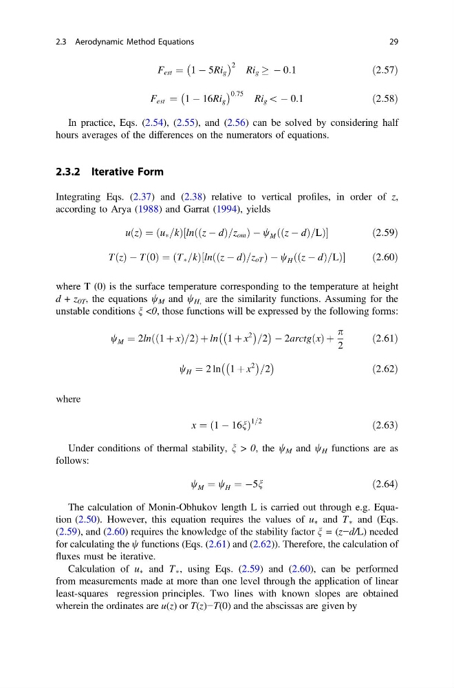
F est ¼ 1 À 5Ri g
À
Á 2 Ri g ! À 0:1
ð2:57Þ
F est ¼ 1 À 16Ri g
À
Á 0:75 Ri g \ À 0:1
ð2:58Þ
In practice, Eqs. (2.54), (2.55), and (2.56) can be solved by considering half
hours averages of the differences on the numerators of equations.
2.3.2 Iterative Form
Integrating Eqs. (2.37) and (2.38) relative to vertical profiles, in order of z,
according to Arya (1988) and Garrat (1994), yields
u z
ð Þ ¼ u à =k
ð
Þln z À d
ð
Þ=z om
ð
ÞÀw M z À d
ð
Þ=L
ð
Þ
½
Š
ð 2:59Þ
T z
ð Þ À T 0
ð Þ ¼ T Ã =k
ð
Þln z À d
ð
Þ=z oT
ð
ÞÀw H z À d
ð
Þ=L
ð
Þ
½
Š
ð 2:60Þ
where T (0) is the surface temperature corresponding to the temperature at height
d + z 0T , the equations w M and w H, are the similarity functions. Assuming for the
unstable conditions n <0, those functions will be expressed by the following forms:
w M ¼ 2ln 1 þ x
ð
Þ=2
ð
Þþln 1 þ x
2
À
Á =2
À
Á À 2arctg x
ð Þ þ
p
2
ð2:61Þ
w H ¼ 2 ln 1 þ x
2
À
Á =2
À
Á
ð2:62Þ
where
x ¼ ð1 À 16nÞ
1=2
ð2:63Þ
Under conditions of thermal stability, n > 0, the w M and w H functions are as
follows:
w M ¼ w H ¼ À5n
ð2:64Þ
The calculation of Monin-Obhukov length L is carried out through e.g. Equation (2.50). However, this equation requires the values of u à and T à and (Eqs.
(2.59), and (2.60) requires the knowledge of the stability factor n = (z−d/L) needed
for calculating the w functions (Eqs. (2.61) and (2.62)). Therefore, the calculation of
fluxes must be iterative.
Calculation of u à and T à , using Eqs. (2.59) and (2.60), can be performed
from measurements made at more than one level through the application of linear
least-squares regression principles. Two lines with known slopes are obtained
wherein the ordinates are u(z) or T(z)−T(0) and the abscissas are given by
2.3 Aerodynamic Method Equations
29