

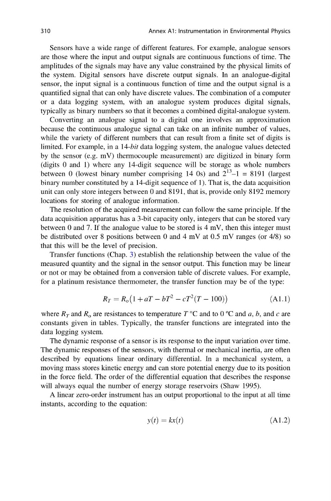
Sensors have a wide range of different features. For example, analogue sensors
are those where the input and output signals are continuous functions of time. The
amplitudes of the signals may have any value constrained by the physical limits of
the system. Digital sensors have discrete output signals. In an analogue-digital
sensor, the input signal is a continuous function of time and the output signal is a
quantified signal that can only have discrete values. The combination of a computer
or a data logging system, with an analogue system produces digital signals,
typically as binary numbers so that it becomes a combined digital-analogue system.
Converting an analogue signal to a digital one involves an approximation
because the continuous analogue signal can take on an infinite number of values,
while the variety of different numbers that can result from a finite set of digits is
limited. For example, in a 14-bit data logging system, the analogue values detected
by the sensor (e.g. mV) thermocouple measurement) are digitized in binary form
(digits 0 and 1) where any 14-digit sequence will be storage as whole numbers
between 0 (lowest binary number comprising 14 0s) and 2
13
–1 = 8191 (largest
binary number constituted by a 14-digit sequence of 1). That is, the data acquisition
unit can only store integers between 0 and 8191, that is, provide only 8192 memory
locations for storing of analogue information.
The resolution of the acquired measurement can follow the same principle. If the
data acquisition apparatus has a 3-bit capacity only, integers that can be stored vary
between 0 and 7. If the analogue value to be stored is 4 mV, then this integer must
be distributed over 8 positions between 0 and 4 mV at 0.5 mV ranges (or 4/8) so
that this will be the level of precision.
Transfer functions (Chap. 3) establish the relationship between the value of the
measured quantity and the signal in the sensor output. This function may be linear
or not or may be obtained from a conversion table of discrete values. For example,
for a platinum resistance thermometer, the transfer function may be of the type:
R T ¼ R o 1 þ aT À bT
2
À cT
2
ðT À 100Þ
À
Á
ðA1:1Þ
where R T and R o are resistances to temperature T °C and to 0 ºC and a, b, and c are
constants given in tables. Typically, the transfer functions are integrated into the
data logging system.
The dynamic response of a sensor is its response to the input variation over time.
The dynamic responses of the sensors, with thermal or mechanical inertia, are often
described by equations linear ordinary differential. In a mechanical system, a
moving mass stores kinetic energy and can store potential energy due to its position
in the force field. The order of the differential equation that describes the response
will always equal the number of energy storage reservoirs (Shaw 1995).
A linear zero-order instrument has an output proportional to the input at all time
instants, according to the equation:
yðtÞ ¼ kxðtÞ
ð A1:2Þ
310
Annex A1: Instrumentation in Environmental Physics
are those where the input and output signals are continuous functions of time. The
amplitudes of the signals may have any value constrained by the physical limits of
the system. Digital sensors have discrete output signals. In an analogue-digital
sensor, the input signal is a continuous function of time and the output signal is a
quantified signal that can only have discrete values. The combination of a computer
or a data logging system, with an analogue system produces digital signals,
typically as binary numbers so that it becomes a combined digital-analogue system.
Converting an analogue signal to a digital one involves an approximation
because the continuous analogue signal can take on an infinite number of values,
while the variety of different numbers that can result from a finite set of digits is
limited. For example, in a 14-bit data logging system, the analogue values detected
by the sensor (e.g. mV) thermocouple measurement) are digitized in binary form
(digits 0 and 1) where any 14-digit sequence will be storage as whole numbers
between 0 (lowest binary number comprising 14 0s) and 2
13
–1 = 8191 (largest
binary number constituted by a 14-digit sequence of 1). That is, the data acquisition
unit can only store integers between 0 and 8191, that is, provide only 8192 memory
locations for storing of analogue information.
The resolution of the acquired measurement can follow the same principle. If the
data acquisition apparatus has a 3-bit capacity only, integers that can be stored vary
between 0 and 7. If the analogue value to be stored is 4 mV, then this integer must
be distributed over 8 positions between 0 and 4 mV at 0.5 mV ranges (or 4/8) so
that this will be the level of precision.
Transfer functions (Chap. 3) establish the relationship between the value of the
measured quantity and the signal in the sensor output. This function may be linear
or not or may be obtained from a conversion table of discrete values. For example,
for a platinum resistance thermometer, the transfer function may be of the type:
R T ¼ R o 1 þ aT À bT
2
À cT
2
ðT À 100Þ
À
Á
ðA1:1Þ
where R T and R o are resistances to temperature T °C and to 0 ºC and a, b, and c are
constants given in tables. Typically, the transfer functions are integrated into the
data logging system.
The dynamic response of a sensor is its response to the input variation over time.
The dynamic responses of the sensors, with thermal or mechanical inertia, are often
described by equations linear ordinary differential. In a mechanical system, a
moving mass stores kinetic energy and can store potential energy due to its position
in the force field. The order of the differential equation that describes the response
will always equal the number of energy storage reservoirs (Shaw 1995).
A linear zero-order instrument has an output proportional to the input at all time
instants, according to the equation:
yðtÞ ¼ kxðtÞ
ð A1:2Þ
310
Annex A1: Instrumentation in Environmental Physics