

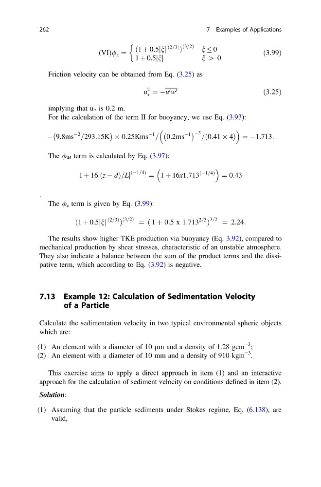
(VIÞ/ e ¼ ð1 þ 0.5 n
j j
ð2=3Þ
Þ
ð3=2Þ
n 0
1 þ 0.5 n
j j
n [ 0
&
ð3:99Þ
Friction velocity can be obtained from Eq. (3.25) as
u
2
à ¼ Àu 0 w 0
ð3:25Þ
implying that u * is 0.2 m.
For the calculation of the term II for buoyancy, we use Eq. (3.93):
À 9:8ms
À2
=293:15K
À
Á Â 0:25Kms
À1
= 0:2ms
À1
À
Á À3 =ð0:41 Â 4Þ
¼ À1:713:
The / M term is calculated by Eq. (3.97):
1 þ 16 z À d
ð
Þ=L
j
j
ðÀ1=4Þ ¼ 1 þ 16x1:713
À1=4
ð
Þ
¼ 0:43
.
The / e term is given by Eq. (3.99):
ð1 þ 0.5 n
j j
ð2=3Þ
Þ
ð3=2Þ ¼ ð 1 þ 0:5 x 1:713
2=3
Þ
3=2 ¼ 2:24:
The results show higher TKE production via buoyancy (Eq. 3.92), compared to
mechanical production by shear stresses, characteristic of an unstable atmosphere.
They also indicate a balance between the sum of the product terms and the dissipative term, which according to Eq. (3.92) is negative.
7.13 Example 12: Calculation of Sedimentation Velocity
of a Particle
Calculate the sedimentation velocity in two typical environmental spheric objects
which are:
(1) An element with a diameter of 10 lm and a density of 1.28 gcm
−3 ;
(2) An element with a diameter of 10 mm and a density of 910 kgm
−3 .
This exercise aims to apply a direct approach in item (1) and an interactive
approach for the calculation of sediment velocity on conditions defined in item (2).
Solution:
(1) Assuming that the particle sediments under Stokes regime, Eq. (6.138), are
valid,
262
7 Examples of Applications
j j
ð2=3Þ
Þ
ð3=2Þ
n 0
1 þ 0.5 n
j j
n [ 0
&
ð3:99Þ
Friction velocity can be obtained from Eq. (3.25) as
u
2
à ¼ Àu 0 w 0
ð3:25Þ
implying that u * is 0.2 m.
For the calculation of the term II for buoyancy, we use Eq. (3.93):
À 9:8ms
À2
=293:15K
À
Á Â 0:25Kms
À1
= 0:2ms
À1
À
Á À3 =ð0:41 Â 4Þ
¼ À1:713:
The / M term is calculated by Eq. (3.97):
1 þ 16 z À d
ð
Þ=L
j
j
ðÀ1=4Þ ¼ 1 þ 16x1:713
À1=4
ð
Þ
¼ 0:43
.
The / e term is given by Eq. (3.99):
ð1 þ 0.5 n
j j
ð2=3Þ
Þ
ð3=2Þ ¼ ð 1 þ 0:5 x 1:713
2=3
Þ
3=2 ¼ 2:24:
The results show higher TKE production via buoyancy (Eq. 3.92), compared to
mechanical production by shear stresses, characteristic of an unstable atmosphere.
They also indicate a balance between the sum of the product terms and the dissipative term, which according to Eq. (3.92) is negative.
7.13 Example 12: Calculation of Sedimentation Velocity
of a Particle
Calculate the sedimentation velocity in two typical environmental spheric objects
which are:
(1) An element with a diameter of 10 lm and a density of 1.28 gcm
−3 ;
(2) An element with a diameter of 10 mm and a density of 910 kgm
−3 .
This exercise aims to apply a direct approach in item (1) and an interactive
approach for the calculation of sediment velocity on conditions defined in item (2).
Solution:
(1) Assuming that the particle sediments under Stokes regime, Eq. (6.138), are
valid,
262
7 Examples of Applications