

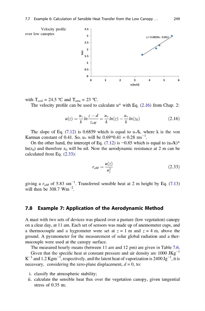
Fig. 7.7 Velocity profile
over low canopies
with T soil = 24.5 ºC and T atm = 23 ºC.
The velocity profile can be used to calculate u* with Eq. (2.16) from Chap. 2:
u z
ð Þ ¼
u Ã
k
ln
z À d
z oM
¼
u Ã
k
ln z
ð Þ À
u Ã
k
ln z 0
ð Þ
ð2:16Þ
The slope of Eq. (7.12) is 0.6859 which is equal to u * /k, where k is the von
Karman constant of 0.41. So, u * will be 0.69*0.41 = 0.28 ms
−1 .
On the other hand, the intercept of Eq. (7.12) is −0.85 which is equal to (u * /k)*
ln(z 0 ) and therefore z 0 will be nil. Now the aerodynamic resistance at 2 m can be
calculated from Eq. (2.33):
r aM ¼
u z
ð Þ
u 2
z
ð2:33Þ
giving a r aM of 5.83 sm
−1 . Transferred sensible heat at 2 m height by Eq. (7.13)
will then be 308.7 Wm
−2
.
7.8 Example 7: Application of the Aerodynamic Method
A mast with two sets of devices was placed over a pasture (low vegetation) canopy
on a clear day, at 11 am. Each set of sensors was made up of anemometer cups, and
a thermocouple and a hygrometer were set at z = 1 m and z = 4 m, above the
ground. A pyranometer for the measurement of solar global radiation and a thermocouple were used at the canopy surface.
The measured hourly means (between 11 am and 12 pm) are given in Table 7.6.
Given that the specific heat at constant pressure and air density are 1000 JKg
−1
K
−1 and 1.2 Kgm
−3 , respectively, and the latent heat of vaporization is 2400 Jg
−1 , it is
necessary, considering the zero-plane displacement, d = 0, to:
i. classify the atmospheric stability;
ii. calculate the sensible heat flux over the vegetation canopy, given tangential
stress of 0.35 m;
7.7 Example 6: Calculation of Sensible Heat Transfer from the Low Canopy …
249
over low canopies
with T soil = 24.5 ºC and T atm = 23 ºC.
The velocity profile can be used to calculate u* with Eq. (2.16) from Chap. 2:
u z
ð Þ ¼
u Ã
k
ln
z À d
z oM
¼
u Ã
k
ln z
ð Þ À
u Ã
k
ln z 0
ð Þ
ð2:16Þ
The slope of Eq. (7.12) is 0.6859 which is equal to u * /k, where k is the von
Karman constant of 0.41. So, u * will be 0.69*0.41 = 0.28 ms
−1 .
On the other hand, the intercept of Eq. (7.12) is −0.85 which is equal to (u * /k)*
ln(z 0 ) and therefore z 0 will be nil. Now the aerodynamic resistance at 2 m can be
calculated from Eq. (2.33):
r aM ¼
u z
ð Þ
u 2
z
ð2:33Þ
giving a r aM of 5.83 sm
−1 . Transferred sensible heat at 2 m height by Eq. (7.13)
will then be 308.7 Wm
−2
.
7.8 Example 7: Application of the Aerodynamic Method
A mast with two sets of devices was placed over a pasture (low vegetation) canopy
on a clear day, at 11 am. Each set of sensors was made up of anemometer cups, and
a thermocouple and a hygrometer were set at z = 1 m and z = 4 m, above the
ground. A pyranometer for the measurement of solar global radiation and a thermocouple were used at the canopy surface.
The measured hourly means (between 11 am and 12 pm) are given in Table 7.6.
Given that the specific heat at constant pressure and air density are 1000 JKg
−1
K
−1 and 1.2 Kgm
−3 , respectively, and the latent heat of vaporization is 2400 Jg
−1 , it is
necessary, considering the zero-plane displacement, d = 0, to:
i. classify the atmospheric stability;
ii. calculate the sensible heat flux over the vegetation canopy, given tangential
stress of 0.35 m;
7.7 Example 6: Calculation of Sensible Heat Transfer from the Low Canopy …
249