

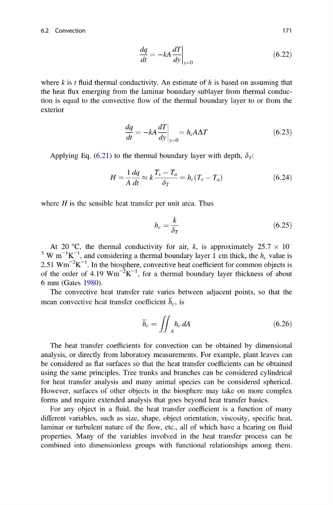
dq
dt
¼ ÀkA
dT
dy
y¼0
ð6:22Þ
where k is t fluid thermal conductivity. An estimate of h is based on assuming that
the heat flux emerging from the laminar boundary sublayer from thermal conduction is equal to the convective flow of the thermal boundary layer to or from the
exterior
dq
dt
¼ ÀkA
dT
dy
y¼0
¼ h c ADT
ð6:23Þ
Applying Eq. (6.21) to the thermal boundary layer with depth, d T :
H ¼
1
A
dq
dt
% k
T s À T a
d T
¼ h c ðT s À T a Þ
ð 6:24Þ
where H is the sensible heat transfer per unit area. Thus
h c ¼
k
d T
ð6:25Þ
At 20 °C, the thermal conductivity for air, k, is approximately 25.7 Â 10
–
3 W m
−1 K
−1 , and considering a thermal boundary layer 1 cm thick, the h c value is
2.51 Wm
−2 K
−1 . In the biosphere, convective heat coefficient for common objects is
of the order of 4.19 Wm
−2 K
−1 , for a thermal boundary layer thickness of about
6 mm (Gates 1980).
The convective heat transfer rate varies between adjacent points, so that the
mean convective heat transfer coefficient h c , is
h c ¼
ZZ
A
h c dA
ð6:26Þ
The heat transfer coefficients for convection can be obtained by dimensional
analysis, or directly from laboratory measurements. For example, plant leaves can
be considered as flat surfaces so that the heat transfer coefficients can be obtained
using the same principles. Tree trunks and branches can be considered cylindrical
for heat transfer analysis and many animal species can be considered spherical.
However, surfaces of other objects in the biosphere may take on more complex
forms and require extended analysis that goes beyond heat transfer basics.
For any object in a fluid, the heat transfer coefficient is a function of many
different variables, such as size, shape, object orientation, viscosity, specific heat,
laminar or turbulent nature of the flow, etc., all of which have a bearing on fluid
properties. Many of the variables involved in the heat transfer process can be
combined into dimensionless groups with functional relationships among them.
6.2 Convection
171
dt
¼ ÀkA
dT
dy
y¼0
ð6:22Þ
where k is t fluid thermal conductivity. An estimate of h is based on assuming that
the heat flux emerging from the laminar boundary sublayer from thermal conduction is equal to the convective flow of the thermal boundary layer to or from the
exterior
dq
dt
¼ ÀkA
dT
dy
y¼0
¼ h c ADT
ð6:23Þ
Applying Eq. (6.21) to the thermal boundary layer with depth, d T :
H ¼
1
A
dq
dt
% k
T s À T a
d T
¼ h c ðT s À T a Þ
ð 6:24Þ
where H is the sensible heat transfer per unit area. Thus
h c ¼
k
d T
ð6:25Þ
At 20 °C, the thermal conductivity for air, k, is approximately 25.7 Â 10
–
3 W m
−1 K
−1 , and considering a thermal boundary layer 1 cm thick, the h c value is
2.51 Wm
−2 K
−1 . In the biosphere, convective heat coefficient for common objects is
of the order of 4.19 Wm
−2 K
−1 , for a thermal boundary layer thickness of about
6 mm (Gates 1980).
The convective heat transfer rate varies between adjacent points, so that the
mean convective heat transfer coefficient h c , is
h c ¼
ZZ
A
h c dA
ð6:26Þ
The heat transfer coefficients for convection can be obtained by dimensional
analysis, or directly from laboratory measurements. For example, plant leaves can
be considered as flat surfaces so that the heat transfer coefficients can be obtained
using the same principles. Tree trunks and branches can be considered cylindrical
for heat transfer analysis and many animal species can be considered spherical.
However, surfaces of other objects in the biosphere may take on more complex
forms and require extended analysis that goes beyond heat transfer basics.
For any object in a fluid, the heat transfer coefficient is a function of many
different variables, such as size, shape, object orientation, viscosity, specific heat,
laminar or turbulent nature of the flow, etc., all of which have a bearing on fluid
properties. Many of the variables involved in the heat transfer process can be
combined into dimensionless groups with functional relationships among them.
6.2 Convection
171