

where F is the corrected flux, F un the uncorrected flux, E evaporation, H sensible
heat flux, ½c mean CO 2 concentration, q V ; q d ; and q water vapor density, dry air,
and standard air, respectively, c p the specific heat at constant pressure and T a the air
temperature in ºK. The expression for closed-circuit systems is slightly different.
The WPL correction is small during seasonal growth and becomes more significant
outside this period (Burba and Anderson 2010). This correction applies to CO 2 fluxes,
evapotranspiration, methane, and ozone, and any other trace atmospheric gas, where
Eq. (3.195) should be applied. The WPL correction for carbon dioxide fluxes will be
about 50%, which is much higher than that for latent heat flux (Leuning et al. 1982). In
very cold environments, open-path analyzers require additional corrections not necessary e.g. in Mediterranean environments (Burba et al. 2008).
(v) An appropriate rotation of coordinates so that the u component coincides with
the wind mean velocity vector, thus canceling the v and w components for
correct application of the eddy covariance method. The mean values of the
vertical component of wind velocity that differ from zero are due to deformation
of streamlines by the ground slope, distortions caused by transducers, or tower
interference. The rotation coordinates can be made before or after averaging
operations (Rannik and Vesala 1999; Foken 2017) discussed in item (vi).
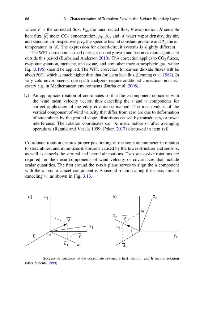
Coordinate rotation ensures proper positioning of the sonic anemometer in relation
to streamlines, and minimizes distortions caused by the tower structure and sensors,
as well as cancels the vertical and lateral air motions. Two successive rotations are
required for the mean components of wind velocity or covariances that include
scalar quantities. The first around the z-axis plane serves to align the u component
with the x-axis to cancel component v. A second rotation along the v-axis aims at
canceling w, as shown in Fig. 3.13.
a)
b)
V
η
V
w
z 1
z 2
y 2
y 1
x 1
u 1
u
y
u 1
u 2
x 2
Fig. 3.13 Successive rotations of the coordinate system, a first rotation, and b second rotation
(after Valente 1999)
86
3 Characterization of Turbulent Flow in the Surface Boundary Layer
heat flux, ½c mean CO 2 concentration, q V ; q d ; and q water vapor density, dry air,
and standard air, respectively, c p the specific heat at constant pressure and T a the air
temperature in ºK. The expression for closed-circuit systems is slightly different.
The WPL correction is small during seasonal growth and becomes more significant
outside this period (Burba and Anderson 2010). This correction applies to CO 2 fluxes,
evapotranspiration, methane, and ozone, and any other trace atmospheric gas, where
Eq. (3.195) should be applied. The WPL correction for carbon dioxide fluxes will be
about 50%, which is much higher than that for latent heat flux (Leuning et al. 1982). In
very cold environments, open-path analyzers require additional corrections not necessary e.g. in Mediterranean environments (Burba et al. 2008).
(v) An appropriate rotation of coordinates so that the u component coincides with
the wind mean velocity vector, thus canceling the v and w components for
correct application of the eddy covariance method. The mean values of the
vertical component of wind velocity that differ from zero are due to deformation
of streamlines by the ground slope, distortions caused by transducers, or tower
interference. The rotation coordinates can be made before or after averaging
operations (Rannik and Vesala 1999; Foken 2017) discussed in item (vi).
Coordinate rotation ensures proper positioning of the sonic anemometer in relation
to streamlines, and minimizes distortions caused by the tower structure and sensors,
as well as cancels the vertical and lateral air motions. Two successive rotations are
required for the mean components of wind velocity or covariances that include
scalar quantities. The first around the z-axis plane serves to align the u component
with the x-axis to cancel component v. A second rotation along the v-axis aims at
canceling w, as shown in Fig. 3.13.
a)
b)
V
η
V
w
z 1
z 2
y 2
y 1
x 1
u 1
u
y
u 1
u 2
x 2
Fig. 3.13 Successive rotations of the coordinate system, a first rotation, and b second rotation
(after Valente 1999)
86
3 Characterization of Turbulent Flow in the Surface Boundary Layer