

A Study to Generate a Weak Order from a Partially Ordered Set, Taken. . .
75
In order to perform the calculation scheme based on Eqs. 8 and 9 the first step is
to select X 1 and X 2 , i.e. the partitioning of set X.
Step 1:
The sets X 1 and X 2 are:
set X 1 : Fe, Zn, Mn, Pb, V, As
set X 2 : Ni, Al, Cd, Cu, Hg
Step2:
The Dom-matrix is:
X 1
X 2
X 1 : 0.361 0.733
X 2 : 0.0
0.48
Remark 1:
Although Dom(X 1 , X 2 ) = 0.733 is less 0.8 the next calculation steps are
documented, just for a demonstration.
Remark 2:
The partitioning selected above is not the only possible one. For example, the
metalloid As is a minimal element. Why not assign As to X 2 ? Let X 2 ’ = X 2 ∪ {As}
and X 1 ’ = X 1 – {As}. Indeed the value of Dom(X 1 ’, X 2 ’) = 0.833 is better than
that of Dom(X 1 , X 2 ) and correspondingly epsav = 0.395. The disadvantage is that
(X 2 ’,≤) leads due to its symmetry to a very high degree of degeneracy: Fe ∼ = Zn, Pb
∼ = V and As ∼ = Al ∼ = Cd ∼ = Cu. Therefore we continue with the partitioning of X into
X 1 and X 2 as given above.
Step 3: Calculation of the averaged ranks by the lattice-theoretical method (De Loof
et al., 2006) due to X 1 and X 2 of step 1.
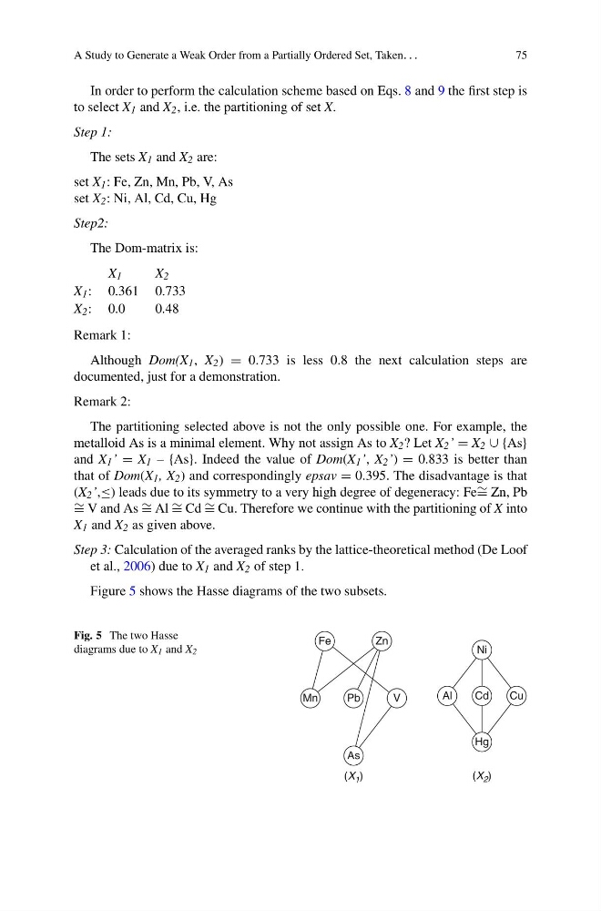
Figure 5 shows the Hasse diagrams of the two subsets.
Fig. 5 The two Hasse
diagrams due to X 1 and X 2
Fe
Zn
V
Pb
Al
Cd
Hg
Cu
Ni
As
Mn
(X 1 )
(X 2 )
75
In order to perform the calculation scheme based on Eqs. 8 and 9 the first step is
to select X 1 and X 2 , i.e. the partitioning of set X.
Step 1:
The sets X 1 and X 2 are:
set X 1 : Fe, Zn, Mn, Pb, V, As
set X 2 : Ni, Al, Cd, Cu, Hg
Step2:
The Dom-matrix is:
X 1
X 2
X 1 : 0.361 0.733
X 2 : 0.0
0.48
Remark 1:
Although Dom(X 1 , X 2 ) = 0.733 is less 0.8 the next calculation steps are
documented, just for a demonstration.
Remark 2:
The partitioning selected above is not the only possible one. For example, the
metalloid As is a minimal element. Why not assign As to X 2 ? Let X 2 ’ = X 2 ∪ {As}
and X 1 ’ = X 1 – {As}. Indeed the value of Dom(X 1 ’, X 2 ’) = 0.833 is better than
that of Dom(X 1 , X 2 ) and correspondingly epsav = 0.395. The disadvantage is that
(X 2 ’,≤) leads due to its symmetry to a very high degree of degeneracy: Fe ∼ = Zn, Pb
∼ = V and As ∼ = Al ∼ = Cd ∼ = Cu. Therefore we continue with the partitioning of X into
X 1 and X 2 as given above.
Step 3: Calculation of the averaged ranks by the lattice-theoretical method (De Loof
et al., 2006) due to X 1 and X 2 of step 1.
Figure 5 shows the Hasse diagrams of the two subsets.
Fig. 5 The two Hasse
diagrams due to X 1 and X 2
Fe
Zn
V
Pb
Al
Cd
Hg
Cu
Ni
As
Mn
(X 1 )
(X 2 )