

Uncertainty in Weights for Composite Indicators Generated by Weighted Sums
47
where x (i, j) is the value of the i
th object and the j
th indicator (j = 1, .., m)
(1)
x (i1) ≤ x (i2) : ⇐⇒ (x (i1, 1) , . . . , x (i1, m)) ≤
x (i2, 1) , . . . .x
i2, m
(2)
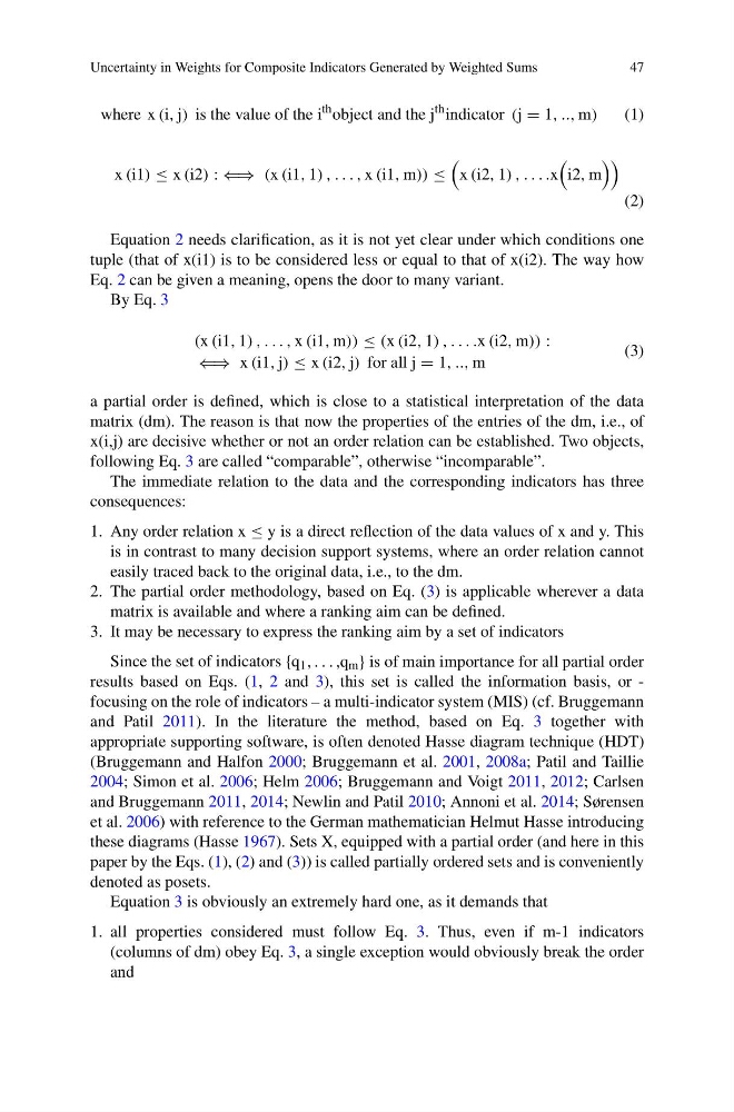
Equation 2 needs clarification, as it is not yet clear under which conditions one
tuple (that of x(i1) is to be considered less or equal to that of x(i2). The way how
Eq. 2 can be given a meaning, opens the door to many variant.
By Eq. 3
(x (i1, 1) , . . . , x (i1, m)) ≤ (x (i2, 1) , . . . .x (i2, m)) :
⇐⇒ x (i1, j) ≤ x (i2, j) for all j = 1, .., m
(3)
a partial order is defined, which is close to a statistical interpretation of the data
matrix (dm). The reason is that now the properties of the entries of the dm, i.e., of
x(i,j) are decisive whether or not an order relation can be established. Two objects,
following Eq. 3 are called “comparable”, otherwise “incomparable”.
The immediate relation to the data and the corresponding indicators has three
consequences:
1. Any order relation x ≤ y is a direct reflection of the data values of x and y. This
is in contrast to many decision support systems, where an order relation cannot
easily traced back to the original data, i.e., to the dm.
2. The partial order methodology, based on Eq. (3) is applicable wherever a data
matrix is available and where a ranking aim can be defined.
3. It may be necessary to express the ranking aim by a set of indicators
Since the set of indicators {q 1 , . . . ,q m } is of main importance for all partial order
results based on Eqs. (1, 2 and 3), this set is called the information basis, or -
focusing on the role of indicators – a multi-indicator system (MIS) (cf. Bruggemann
and Patil 2011). In the literature the method, based on Eq. 3 together with
appropriate supporting software, is often denoted Hasse diagram technique (HDT)
(Bruggemann and Halfon 2000; Bruggemann et al. 2001, 2008a; Patil and Taillie
2004; Simon et al. 2006; Helm 2006; Bruggemann and Voigt 2011, 2012; Carlsen
and Bruggemann 2011, 2014; Newlin and Patil 2010; Annoni et al. 2014; Sørensen
et al. 2006) with reference to the German mathematician Helmut Hasse introducing
these diagrams (Hasse 1967). Sets X, equipped with a partial order (and here in this
paper by the Eqs. (1), (2) and (3)) is called partially ordered sets and is conveniently
denoted as posets.
Equation 3 is obviously an extremely hard one, as it demands that
1. all properties considered must follow Eq. 3. Thus, even if m-1 indicators
(columns of dm) obey Eq. 3, a single exception would obviously break the order
and
47
where x (i, j) is the value of the i
th object and the j
th indicator (j = 1, .., m)
(1)
x (i1) ≤ x (i2) : ⇐⇒ (x (i1, 1) , . . . , x (i1, m)) ≤
x (i2, 1) , . . . .x
i2, m
(2)
Equation 2 needs clarification, as it is not yet clear under which conditions one
tuple (that of x(i1) is to be considered less or equal to that of x(i2). The way how
Eq. 2 can be given a meaning, opens the door to many variant.
By Eq. 3
(x (i1, 1) , . . . , x (i1, m)) ≤ (x (i2, 1) , . . . .x (i2, m)) :
⇐⇒ x (i1, j) ≤ x (i2, j) for all j = 1, .., m
(3)
a partial order is defined, which is close to a statistical interpretation of the data
matrix (dm). The reason is that now the properties of the entries of the dm, i.e., of
x(i,j) are decisive whether or not an order relation can be established. Two objects,
following Eq. 3 are called “comparable”, otherwise “incomparable”.
The immediate relation to the data and the corresponding indicators has three
consequences:
1. Any order relation x ≤ y is a direct reflection of the data values of x and y. This
is in contrast to many decision support systems, where an order relation cannot
easily traced back to the original data, i.e., to the dm.
2. The partial order methodology, based on Eq. (3) is applicable wherever a data
matrix is available and where a ranking aim can be defined.
3. It may be necessary to express the ranking aim by a set of indicators
Since the set of indicators {q 1 , . . . ,q m } is of main importance for all partial order
results based on Eqs. (1, 2 and 3), this set is called the information basis, or -
focusing on the role of indicators – a multi-indicator system (MIS) (cf. Bruggemann
and Patil 2011). In the literature the method, based on Eq. 3 together with
appropriate supporting software, is often denoted Hasse diagram technique (HDT)
(Bruggemann and Halfon 2000; Bruggemann et al. 2001, 2008a; Patil and Taillie
2004; Simon et al. 2006; Helm 2006; Bruggemann and Voigt 2011, 2012; Carlsen
and Bruggemann 2011, 2014; Newlin and Patil 2010; Annoni et al. 2014; Sørensen
et al. 2006) with reference to the German mathematician Helmut Hasse introducing
these diagrams (Hasse 1967). Sets X, equipped with a partial order (and here in this
paper by the Eqs. (1), (2) and (3)) is called partially ordered sets and is conveniently
denoted as posets.
Equation 3 is obviously an extremely hard one, as it demands that
1. all properties considered must follow Eq. 3. Thus, even if m-1 indicators
(columns of dm) obey Eq. 3, a single exception would obviously break the order
and