

Assessing Inhomogeneous Indicator-Related Typologies Through the Reverse. . .
39
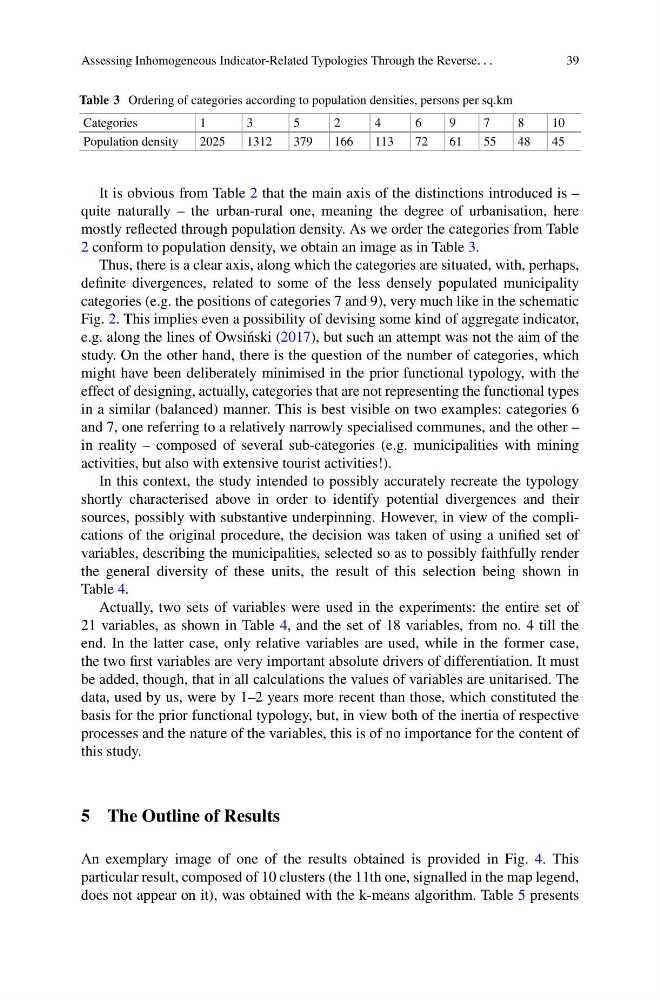
Table 3 Ordering of categories according to population densities, persons per sq.km
Categories
1
3
5
2
4
6
9
7
8
10
Population density
2025
1312
379
166
113
72
61
55
48
45
It is obvious from Table 2 that the main axis of the distinctions introduced is –
quite naturally – the urban-rural one, meaning the degree of urbanisation, here
mostly reflected through population density. As we order the categories from Table
2 conform to population density, we obtain an image as in Table 3.
Thus, there is a clear axis, along which the categories are situated, with, perhaps,
definite divergences, related to some of the less densely populated municipality
categories (e.g. the positions of categories 7 and 9), very much like in the schematic
Fig. 2. This implies even a possibility of devising some kind of aggregate indicator,
e.g. along the lines of Owsi´ nski (2017), but such an attempt was not the aim of the
study. On the other hand, there is the question of the number of categories, which
might have been deliberately minimised in the prior functional typology, with the
effect of designing, actually, categories that are not representing the functional types
in a similar (balanced) manner. This is best visible on two examples: categories 6
and 7, one referring to a relatively narrowly specialised communes, and the other –
in reality – composed of several sub-categories (e.g. municipalities with mining
activities, but also with extensive tourist activities!).
In this context, the study intended to possibly accurately recreate the typology
shortly characterised above in order to identify potential divergences and their
sources, possibly with substantive underpinning. However, in view of the complications of the original procedure, the decision was taken of using a unified set of
variables, describing the municipalities, selected so as to possibly faithfully render
the general diversity of these units, the result of this selection being shown in
Table 4.
Actually, two sets of variables were used in the experiments: the entire set of
21 variables, as shown in Table 4, and the set of 18 variables, from no. 4 till the
end. In the latter case, only relative variables are used, while in the former case,
the two first variables are very important absolute drivers of differentiation. It must
be added, though, that in all calculations the values of variables are unitarised. The
data, used by us, were by 1–2 years more recent than those, which constituted the
basis for the prior functional typology, but, in view both of the inertia of respective
processes and the nature of the variables, this is of no importance for the content of
this study.
5 The Outline of Results
An exemplary image of one of the results obtained is provided in Fig. 4. This
particular result, composed of 10 clusters (the 11th one, signalled in the map legend,
does not appear on it), was obtained with the k-means algorithm. Table 5 presents
39
Table 3 Ordering of categories according to population densities, persons per sq.km
Categories
1
3
5
2
4
6
9
7
8
10
Population density
2025
1312
379
166
113
72
61
55
48
45
It is obvious from Table 2 that the main axis of the distinctions introduced is –
quite naturally – the urban-rural one, meaning the degree of urbanisation, here
mostly reflected through population density. As we order the categories from Table
2 conform to population density, we obtain an image as in Table 3.
Thus, there is a clear axis, along which the categories are situated, with, perhaps,
definite divergences, related to some of the less densely populated municipality
categories (e.g. the positions of categories 7 and 9), very much like in the schematic
Fig. 2. This implies even a possibility of devising some kind of aggregate indicator,
e.g. along the lines of Owsi´ nski (2017), but such an attempt was not the aim of the
study. On the other hand, there is the question of the number of categories, which
might have been deliberately minimised in the prior functional typology, with the
effect of designing, actually, categories that are not representing the functional types
in a similar (balanced) manner. This is best visible on two examples: categories 6
and 7, one referring to a relatively narrowly specialised communes, and the other –
in reality – composed of several sub-categories (e.g. municipalities with mining
activities, but also with extensive tourist activities!).
In this context, the study intended to possibly accurately recreate the typology
shortly characterised above in order to identify potential divergences and their
sources, possibly with substantive underpinning. However, in view of the complications of the original procedure, the decision was taken of using a unified set of
variables, describing the municipalities, selected so as to possibly faithfully render
the general diversity of these units, the result of this selection being shown in
Table 4.
Actually, two sets of variables were used in the experiments: the entire set of
21 variables, as shown in Table 4, and the set of 18 variables, from no. 4 till the
end. In the latter case, only relative variables are used, while in the former case,
the two first variables are very important absolute drivers of differentiation. It must
be added, though, that in all calculations the values of variables are unitarised. The
data, used by us, were by 1–2 years more recent than those, which constituted the
basis for the prior functional typology, but, in view both of the inertia of respective
processes and the nature of the variables, this is of no importance for the content of
this study.
5 The Outline of Results
An exemplary image of one of the results obtained is provided in Fig. 4. This
particular result, composed of 10 clusters (the 11th one, signalled in the map legend,
does not appear on it), was obtained with the k-means algorithm. Table 5 presents