

1.8. THE TANGENT LINE APPROXIMATION
81
L ′ (x) = f ′ (a) for every value of x, and specifically L ′ (a) = f ′ (a). Therefore, we see that
L is a linear function that has both the same value and the same slope as the function f
at the point (a, f (a)).
In situations where we know the linear approximation y = L(x), we therefore know
the original function’s value and slope at the point of tangency. What remains unknown,
however, is the shape of the function f at the point of tangency. There are essentially four
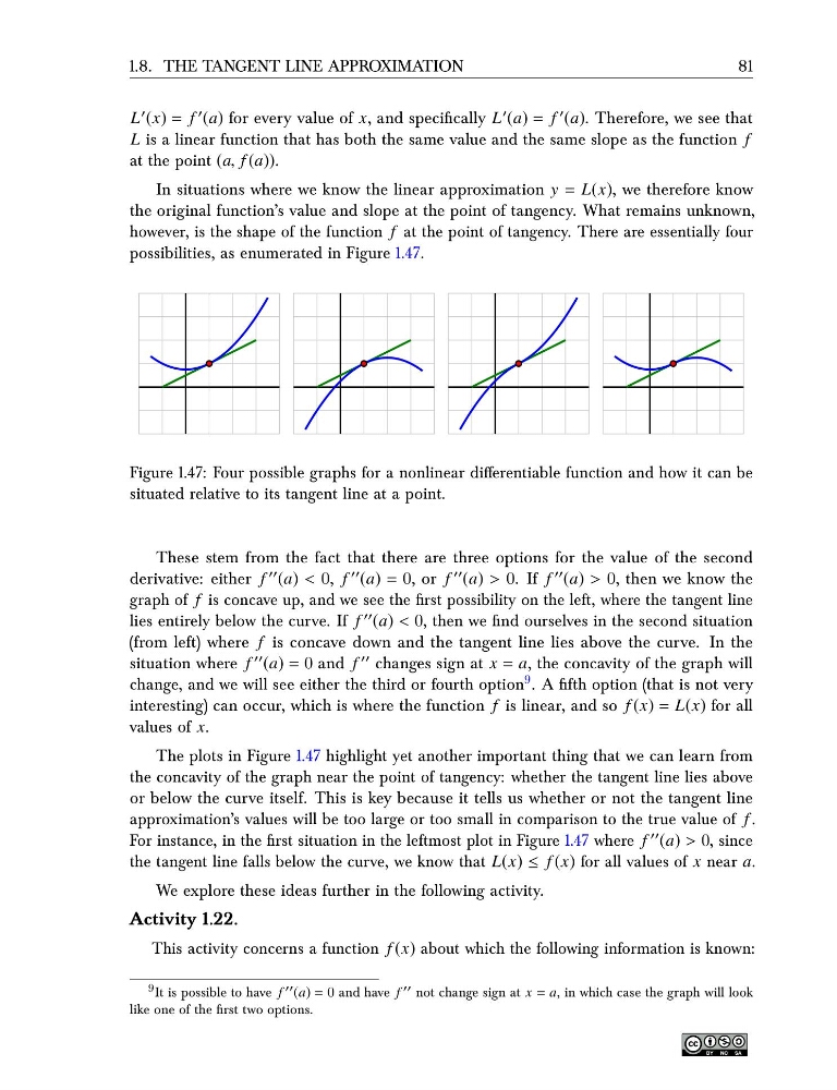
possibilities, as enumerated in Figure 1.47.
Figure 1.47: Four possible graphs for a nonlinear differentiable function and how it can be
situated relative to its tangent line at a point.
These stem from the fact that there are three options for the value of the second
derivative: either f ′′ (a) < 0, f ′′ (a) = 0, or f ′′ (a) > 0. If f ′′ (a) > 0, then we know the
graph of f is concave up, and we see the first possibility on the left, where the tangent line
lies entirely below the curve. If f ′′ (a) < 0, then we find ourselves in the second situation
(from left) where f is concave down and the tangent line lies above the curve. In the
situation where f ′′ (a) = 0 and f ′′ changes sign at x = a, the concavity of the graph will
change, and we will see either the third or fourth option 9 . A fifth option (that is not very
interesting) can occur, which is where the function f is linear, and so f (x) = L(x) for all
values of x.
The plots in Figure 1.47 highlight yet another important thing that we can learn from
the concavity of the graph near the point of tangency: whether the tangent line lies above
or below the curve itself. This is key because it tells us whether or not the tangent line
approximation’s values will be too large or too small in comparison to the true value of f .
For instance, in the first situation in the leftmost plot in Figure 1.47 where f ′′ (a) > 0, since
the tangent line falls below the curve, we know that L(x) ≤ f (x) for all values of x near a.
We explore these ideas further in the following activity.
Activity 1.22.
This activity concerns a function f (x) about which the following information is known:
9 It is possible to have f ′′ (a) = 0 and have f ′′ not change sign at x = a, in which case the graph will look
like one of the first two options.
81
L ′ (x) = f ′ (a) for every value of x, and specifically L ′ (a) = f ′ (a). Therefore, we see that
L is a linear function that has both the same value and the same slope as the function f
at the point (a, f (a)).
In situations where we know the linear approximation y = L(x), we therefore know
the original function’s value and slope at the point of tangency. What remains unknown,
however, is the shape of the function f at the point of tangency. There are essentially four
possibilities, as enumerated in Figure 1.47.
Figure 1.47: Four possible graphs for a nonlinear differentiable function and how it can be
situated relative to its tangent line at a point.
These stem from the fact that there are three options for the value of the second
derivative: either f ′′ (a) < 0, f ′′ (a) = 0, or f ′′ (a) > 0. If f ′′ (a) > 0, then we know the
graph of f is concave up, and we see the first possibility on the left, where the tangent line
lies entirely below the curve. If f ′′ (a) < 0, then we find ourselves in the second situation
(from left) where f is concave down and the tangent line lies above the curve. In the
situation where f ′′ (a) = 0 and f ′′ changes sign at x = a, the concavity of the graph will
change, and we will see either the third or fourth option 9 . A fifth option (that is not very
interesting) can occur, which is where the function f is linear, and so f (x) = L(x) for all
values of x.
The plots in Figure 1.47 highlight yet another important thing that we can learn from
the concavity of the graph near the point of tangency: whether the tangent line lies above
or below the curve itself. This is key because it tells us whether or not the tangent line
approximation’s values will be too large or too small in comparison to the true value of f .
For instance, in the first situation in the leftmost plot in Figure 1.47 where f ′′ (a) > 0, since
the tangent line falls below the curve, we know that L(x) ≤ f (x) for all values of x near a.
We explore these ideas further in the following activity.
Activity 1.22.
This activity concerns a function f (x) about which the following information is known:
9 It is possible to have f ′′ (a) = 0 and have f ′′ not change sign at x = a, in which case the graph will look
like one of the first two options.