

46
1.5. INTERPRETING, ESTIMATING, AND USING THE DERIVATIVE
find that
f
′ (2) ≈
0.75 + 0.375
2
= 0.5625.
The intuitive approach to average the two estimates found in Example 1.4 is in fact the
best possible estimate to f ′ (2) when we have just two function values for f on opposite
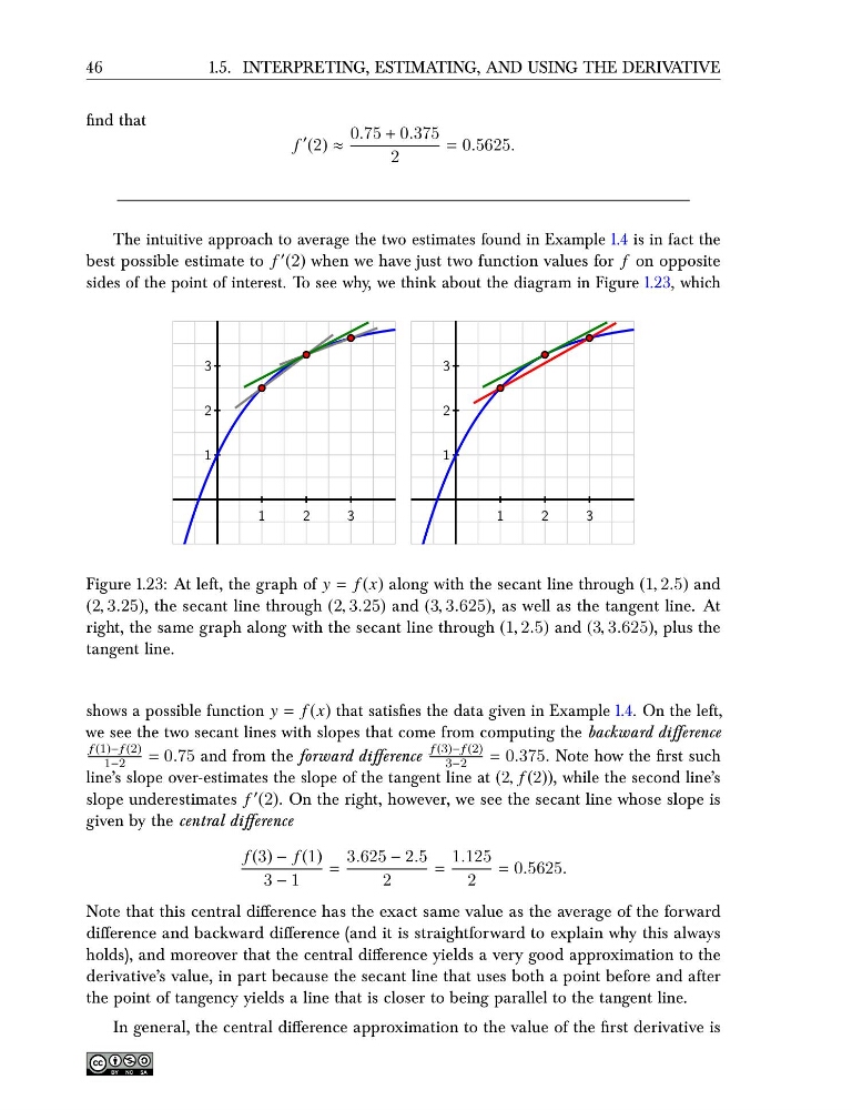
sides of the point of interest. To see why, we think about the diagram in Figure 1.23, which
1
2
3
1
2
3
1
2
3
1
2
3
Figure 1.23: At left, the graph of y = f (x) along with the secant line through (1, 2.5) and
(2, 3.25), the secant line through (2, 3.25) and (3, 3.625), as well as the tangent line. At
right, the same graph along with the secant line through (1, 2.5) and (3, 3.625), plus the
tangent line.
shows a possible function y = f (x) that satisfies the data given in Example 1.4. On the left,
we see the two secant lines with slopes that come from computing the backward difference
f (1)− f (2)
1−2
= 0.75 and from the forward difference
f (3)− f (2)
3−2
= 0.375. Note how the first such
line’s slope over-estimates the slope of the tangent line at (2, f (2)), while the second line’s
slope underestimates f ′ (2). On the right, however, we see the secant line whose slope is
given by the central difference
f (3) − f (1)
3 − 1
=
3.625 − 2.5
2
=
1.125
2
= 0.5625.
Note that this central difference has the exact same value as the average of the forward
difference and backward difference (and it is straightforward to explain why this always
holds), and moreover that the central difference yields a very good approximation to the
derivative’s value, in part because the secant line that uses both a point before and after
the point of tangency yields a line that is closer to being parallel to the tangent line.
In general, the central difference approximation to the value of the first derivative is
1.5. INTERPRETING, ESTIMATING, AND USING THE DERIVATIVE
find that
f
′ (2) ≈
0.75 + 0.375
2
= 0.5625.
The intuitive approach to average the two estimates found in Example 1.4 is in fact the
best possible estimate to f ′ (2) when we have just two function values for f on opposite
sides of the point of interest. To see why, we think about the diagram in Figure 1.23, which
1
2
3
1
2
3
1
2
3
1
2
3
Figure 1.23: At left, the graph of y = f (x) along with the secant line through (1, 2.5) and
(2, 3.25), the secant line through (2, 3.25) and (3, 3.625), as well as the tangent line. At
right, the same graph along with the secant line through (1, 2.5) and (3, 3.625), plus the
tangent line.
shows a possible function y = f (x) that satisfies the data given in Example 1.4. On the left,
we see the two secant lines with slopes that come from computing the backward difference
f (1)− f (2)
1−2
= 0.75 and from the forward difference
f (3)− f (2)
3−2
= 0.375. Note how the first such
line’s slope over-estimates the slope of the tangent line at (2, f (2)), while the second line’s
slope underestimates f ′ (2). On the right, however, we see the secant line whose slope is
given by the central difference
f (3) − f (1)
3 − 1
=
3.625 − 2.5
2
=
1.125
2
= 0.5625.
Note that this central difference has the exact same value as the average of the forward
difference and backward difference (and it is straightforward to explain why this always
holds), and moreover that the central difference yields a very good approximation to the
derivative’s value, in part because the secant line that uses both a point before and after
the point of tangency yields a line that is closer to being parallel to the tangent line.
In general, the central difference approximation to the value of the first derivative is