

1.4. THE DERIVATIVE FUNCTION
41
(b) Use a graphing utility to plot both y = g(x) and your result for y = g ′ (x); does
your formula for g ′ (x) generate the graph you expected?
(c) Use the limit definition of the derivative to find a formula for p ′ (x) where
p(x) = 5x 2 − 4x + 12.
(d) Compare and contrast the formulas for g ′ (x) and p ′ (x) you have found. How
do the constants 5, 4, 12, and 3 affect the results?
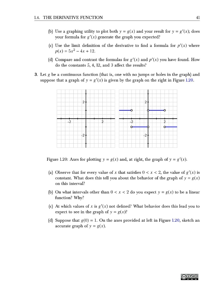
3. Let g be a continuous function (that is, one with no jumps or holes in the graph) and
suppose that a graph of y = g ′ (x) is given by the graph on the right in Figure 1.20.
-2
2
-2
2
-2
2
-2
2
Figure 1.20: Axes for plotting y = g(x) and, at right, the graph of y = g ′ (x).
(a) Observe that for every value of x that satisfies 0 < x < 2, the value of g ′ (x) is
constant. What does this tell you about the behavior of the graph of y = g(x)
on this interval?
(b) On what intervals other than 0 < x < 2 do you expect y = g(x) to be a linear
function? Why?
(c) At which values of x is g ′ (x) not defined? What behavior does this lead you to
expect to see in the graph of y = g(x)?
(d) Suppose that g(0) = 1. On the axes provided at left in Figure 1.20, sketch an
accurate graph of y = g(x).
41
(b) Use a graphing utility to plot both y = g(x) and your result for y = g ′ (x); does
your formula for g ′ (x) generate the graph you expected?
(c) Use the limit definition of the derivative to find a formula for p ′ (x) where
p(x) = 5x 2 − 4x + 12.
(d) Compare and contrast the formulas for g ′ (x) and p ′ (x) you have found. How
do the constants 5, 4, 12, and 3 affect the results?
3. Let g be a continuous function (that is, one with no jumps or holes in the graph) and
suppose that a graph of y = g ′ (x) is given by the graph on the right in Figure 1.20.
-2
2
-2
2
-2
2
-2
2
Figure 1.20: Axes for plotting y = g(x) and, at right, the graph of y = g ′ (x).
(a) Observe that for every value of x that satisfies 0 < x < 2, the value of g ′ (x) is
constant. What does this tell you about the behavior of the graph of y = g(x)
on this interval?
(b) On what intervals other than 0 < x < 2 do you expect y = g(x) to be a linear
function? Why?
(c) At which values of x is g ′ (x) not defined? What behavior does this lead you to
expect to see in the graph of y = g(x)?
(d) Suppose that g(0) = 1. On the axes provided at left in Figure 1.20, sketch an
accurate graph of y = g(x).